Week 1, Session 3 — Data types, tidy data, accuracy and precision

Course 1 — #courses

R. Heller

Note

Workflow labs use the variant template: Goal → Approach → Execution → Check → Report.

Learning objectives

• Classify a variable as nominal, ordinal, interval, or ratio and explain why the distinction dictates what summaries are legal.
• Reshape a rectangular dataset between wide and long form with pivot_longer() and pivot_wider().
• Separate accuracy, precision, and bias by simulation, and say why a precise instrument can still be wrong.

Prerequisites

Lab 1.2 (toolchain).

Background

Statistics is largely the study of variation, and variation must be measured. Before we calculate anything we need to say what kind of variable we are looking at. A nominal variable labels groups without order. An ordinal variable orders them but does not quantify the distance between them. Interval and ratio variables do quantify distances, and ratio variables have a true zero. Tools that average an ordinal variable or compute a standard deviation on a category code produce numbers, but not answers.

Tidy data is a convention, not a requirement, but adopting it pays immediate dividends: every variable gets a column, every observation a row, and every value a cell. Real datasets arrive in other shapes, so a large part of the job is reshaping them until they conform. The tools are pivot_longer() and pivot_wider(), and they are the two functions you will use most often in a working week.

The accuracy/precision/bias triangle is borrowed from measurement theory. Accuracy is how close a measurement is to truth on average. Precision is how tightly repeated measurements cluster. Bias is a systematic offset from truth. An instrument can be precise but biased (tight cluster off-target), accurate but imprecise (wide cluster centred on truth), or — the goal — both.

Setup

library(tidyverse)
set.seed(42)
theme_set(theme_minimal(base_size = 12))

1. Goal

Move a small simulated clinical dataset between wide and long forms and quantify accuracy, precision, and bias in a simulated measurement process.

2. Approach

We simulate three repeat measurements of blood pressure on twelve patients at two visits. This is a realistic wide-format dataset with a within-patient structure.

clinic <- tibble(
  id = sprintf("P%02d", 1:12),
  sex = sample(c("F", "M"), 12, replace = TRUE),
  visit1_sbp1 = rnorm(12, 140, 10),
  visit1_sbp2 = rnorm(12, 140, 10),
  visit1_sbp3 = rnorm(12, 140, 10),
  visit2_sbp1 = rnorm(12, 135, 10),
  visit2_sbp2 = rnorm(12, 135, 10),
  visit2_sbp3 = rnorm(12, 135, 10)
)
clinic |> select(id, starts_with("visit1")) |> head(3)

# A tibble: 3 × 4
  id    visit1_sbp1 visit1_sbp2 visit1_sbp3
  <chr>       <dbl>       <dbl>       <dbl>
1 P01          155.        116.        145.
2 P02          139.        153.        147.
3 P03          160.        137.        150.

3. Execution

Reshape to a long form where each row is one reading.

long <- clinic |>
  pivot_longer(
    cols = starts_with("visit"),
    names_to = c("visit", "reading"),
    names_pattern = "visit(\\d)_sbp(\\d)",
    values_to = "sbp"
  ) |>
  mutate(visit = factor(paste0("V", visit)),
         reading = as.integer(reading))
head(long)

# A tibble: 6 × 5
  id    sex   visit reading   sbp
  <chr> <chr> <fct>   <int> <dbl>
1 P01   F     V1          1  155.
2 P01   F     V1          2  116.
3 P01   F     V1          3  145.
4 P01   F     V2          1  143.
5 P01   F     V2          2  136.
6 P01   F     V2          3  138.

long |>
  ggplot(aes(visit, sbp, colour = sex)) +
  geom_jitter(width = 0.1, alpha = 0.6) +
  labs(x = NULL, y = "SBP (mmHg)")

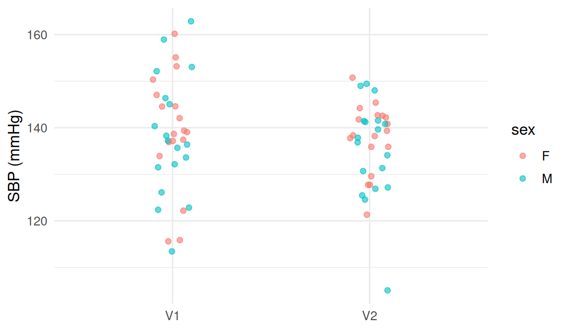
The long format makes it trivial to summarise by visit, by patient, or by visit-and-patient. The same plot in wide format would require custom code for each visit column.

# Collapse three readings per visit to a mean.
by_visit <- long |>
  group_by(id, visit, sex) |>
  summarise(sbp_mean = mean(sbp), .groups = "drop")

# Pivot back to wide if the downstream analysis needs it.
wide <- by_visit |> pivot_wider(names_from = visit, values_from = sbp_mean)
head(wide)

# A tibble: 6 × 4
  id    sex      V1    V2
  <chr> <chr> <dbl> <dbl>
1 P01   F      138.  139.
2 P02   F      146.  137.
3 P03   F      149.  136.
4 P04   F      132.  139.
5 P05   M      145.  119.
6 P06   M      146.  140.

4. Check

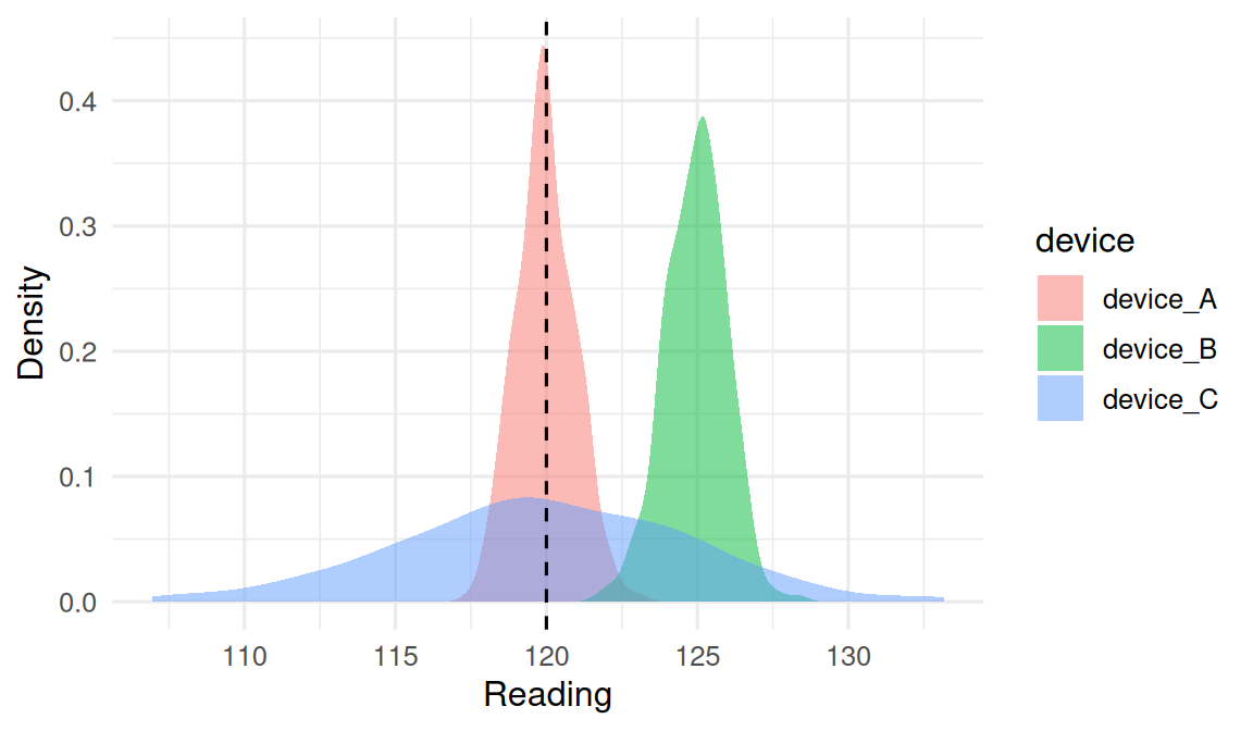
Simulate an instrument with a known truth (say, a calibrated reference of 120) and compare three candidate devices with different accuracy/precision profiles.

truth <- 120
n <- 500
devices <- tibble(
  device_A = rnorm(n, mean = 120, sd = 1),   # accurate & precise
  device_B = rnorm(n, mean = 125, sd = 1),   # precise, biased
  device_C = rnorm(n, mean = 120, sd = 5)    # accurate on average, imprecise
) |>
  pivot_longer(everything(), names_to = "device", values_to = "reading")

summary_table <- devices |>
  group_by(device) |>
  summarise(mean = mean(reading),
            sd = sd(reading),
            bias = mean(reading) - truth,
            rmse = sqrt(mean((reading - truth)^2)))
summary_table

# A tibble: 3 × 5
  device    mean    sd    bias  rmse
  <chr>    <dbl> <dbl>   <dbl> <dbl>
1 device_A  120. 0.974 -0.0280 0.974
2 device_B  125. 1.02   4.95   5.06 
3 device_C  120. 4.83  -0.0819 4.83 

devices |>
  ggplot(aes(reading, fill = device)) +
  geom_density(alpha = 0.5, colour = NA) +
  geom_vline(xintercept = truth, linetype = 2) +
  labs(x = "Reading", y = "Density")

5. Report

In a simulated calibration experiment (n = 500 draws per device), the unbiased precise device had bias = -0.03 mmHg and SD = 0.97; the biased precise device had bias = 4.95 and the same SD; the imprecise unbiased device had bias = -0.08 but SD = 4.83. Root mean squared error captures accuracy overall and is the quantity to minimise.

The lesson is that bias and variance are separately identifiable. A device that is consistent is not necessarily correct, and a device that is correct on average may still be unusable on a single reading.

Use the density plot to anchor the intuition — three distributions, one dashed line at the truth. Ask the audience which device they would use for a single reading, and which for a large calibration study.

Common pitfalls

• Treating ordinal codes (1 = mild, 2 = moderate, 3 = severe) as if the steps were equal.
• Forcing data to stay wide because that is how the spreadsheet happened to arrive.
• Judging a measurement by precision alone. A small SD with a big bias is still the wrong number.
• Using the mean to summarise a nominal variable.

Further reading

• Wickham H (2014), Tidy Data. Journal of Statistical Software.
• Altman DG, Bland JM (1983), Measurement in medicine.

Session info

sessionInfo()

R version 4.4.1 (2024-06-14)
Platform: x86_64-pc-linux-gnu
Running under: Ubuntu 24.04.4 LTS

Matrix products: default
BLAS:   /usr/lib/x86_64-linux-gnu/openblas-pthread/libblas.so.3 
LAPACK: /usr/lib/x86_64-linux-gnu/openblas-pthread/libopenblasp-r0.3.26.so;  LAPACK version 3.12.0

locale:
 [1] LC_CTYPE=C.UTF-8       LC_NUMERIC=C           LC_TIME=C.UTF-8       
 [4] LC_COLLATE=C.UTF-8     LC_MONETARY=C.UTF-8    LC_MESSAGES=C.UTF-8   
 [7] LC_PAPER=C.UTF-8       LC_NAME=C              LC_ADDRESS=C          
[10] LC_TELEPHONE=C         LC_MEASUREMENT=C.UTF-8 LC_IDENTIFICATION=C   

time zone: UTC
tzcode source: system (glibc)

attached base packages:
[1] stats     graphics  grDevices utils     datasets  methods   base     

other attached packages:
 [1] lubridate_1.9.5 forcats_1.0.1   stringr_1.6.0   dplyr_1.2.1    
 [5] purrr_1.2.2     readr_2.2.0     tidyr_1.3.2     tibble_3.3.1   
 [9] ggplot2_4.0.3   tidyverse_2.0.0

loaded via a namespace (and not attached):
 [1] gtable_0.3.6       jsonlite_2.0.0     compiler_4.4.1     tidyselect_1.2.1  
 [5] scales_1.4.0       yaml_2.3.12        fastmap_1.2.0      R6_2.6.1          
 [9] labeling_0.4.3     generics_0.1.4     knitr_1.51         htmlwidgets_1.6.4 
[13] pillar_1.11.1      RColorBrewer_1.1-3 tzdb_0.5.0         rlang_1.2.0       
[17] utf8_1.2.6         stringi_1.8.7      xfun_0.57          S7_0.2.2          
[21] otel_0.2.0         timechange_0.4.0   cli_3.6.6          withr_3.0.2       
[25] magrittr_2.0.5     digest_0.6.39      grid_4.4.1         hms_1.1.4         
[29] lifecycle_1.0.5    vctrs_0.7.3        evaluate_1.0.5     glue_1.8.1        
[33] farver_2.1.2       rmarkdown_2.31     tools_4.4.1        pkgconfig_2.0.3   
[37] htmltools_0.5.9