Week 1, Session 4 — Import, joins, and missingness with dplyr

Course 1 — #courses

R. Heller

Note

Workflow labs use the variant template: Goal → Approach → Execution → Check → Report.

Learning objectives

Use filter(), select(), mutate(), arrange(), group_by(), and summarise() to carry out routine data management with palmerpenguins.
Join two tables on a shared key and explain the difference between inner, left, and anti joins.
Spot, quantify, and respond to missing data without letting NAs propagate silently into a summary.

Prerequisites

Labs 1.2 and 1.3.

Background

The bulk of analytic time is spent moving data from the shape it arrived in to the shape an analysis requires. dplyr names the five verbs you need for most of that work — filter rows, select columns, mutate to create new variables, arrange to sort, summarise with an optional grouping. If you learn these six verbs well you will write less code and hide fewer bugs.

Joins are the other half of data management. Real datasets arrive in pieces — a demographics table, a laboratory table, a follow-up table — that must be connected on a shared identifier. left_join() keeps all rows on the left side; inner_join() keeps only matches; anti_join() returns the rows with no match, which is often where data-quality problems live.

Missingness is not rare. A realistic clinical dataset has NAs in at least half its variables, and the NAs are almost never uniformly distributed. The first question to ask of any new dataset is how much is missing, and where? The second is why? Missing-completely-at- random, missing-at-random, and missing-not-at-random are three distinct problems with different consequences for the analysis.

Setup

library(tidyverse)
library(palmerpenguins)
set.seed(42)
theme_set(theme_minimal(base_size = 12))

1. Goal

Reshape the penguins dataset with the standard dplyr verbs, join a derived table back on, and describe the pattern of missingness.

2. Approach

glimpse(penguins)

Rows: 344
Columns: 8
$ species           <fct> Adelie, Adelie, Adelie, Adelie, Adelie, Adelie, Adel…
$ island            <fct> Torgersen, Torgersen, Torgersen, Torgersen, Torgerse…
$ bill_length_mm    <dbl> 39.1, 39.5, 40.3, NA, 36.7, 39.3, 38.9, 39.2, 34.1, …
$ bill_depth_mm     <dbl> 18.7, 17.4, 18.0, NA, 19.3, 20.6, 17.8, 19.6, 18.1, …
$ flipper_length_mm <int> 181, 186, 195, NA, 193, 190, 181, 195, 193, 190, 186…
$ body_mass_g       <int> 3750, 3800, 3250, NA, 3450, 3650, 3625, 4675, 3475, …
$ sex               <fct> male, female, female, NA, female, male, female, male…
$ year              <int> 2007, 2007, 2007, 2007, 2007, 2007, 2007, 2007, 2007…

# Standard five verbs.
penguins |>
  filter(!is.na(body_mass_g)) |>
  select(species, sex, bill_length_mm, body_mass_g) |>
  mutate(mass_kg = body_mass_g / 1000) |>
  arrange(desc(mass_kg)) |>
  head(5)

# A tibble: 5 × 5
  species sex   bill_length_mm body_mass_g mass_kg
  <fct>   <fct>          <dbl>       <int>   <dbl>
1 Gentoo  male            49.2        6300    6.3 
2 Gentoo  male            59.6        6050    6.05
3 Gentoo  male            51.1        6000    6   
4 Gentoo  male            48.8        6000    6   
5 Gentoo  male            45.2        5950    5.95

# group_by + summarise: the grammar of a Table 1 row.
species_summary <- penguins |>
  group_by(species, sex) |>
  summarise(
    n    = n(),
    mean_mass = mean(body_mass_g, na.rm = TRUE),
    sd_mass   = sd(body_mass_g,   na.rm = TRUE),
    .groups = "drop"
  )
species_summary

# A tibble: 8 × 5
  species   sex        n mean_mass sd_mass
  <fct>     <fct>  <int>     <dbl>   <dbl>
1 Adelie    female    73     3369.    269.
2 Adelie    male      73     4043.    347.
3 Adelie    <NA>       6     3540     477.
4 Chinstrap female    34     3527.    285.
5 Chinstrap male      34     3939.    362.
6 Gentoo    female    58     4680.    282.
7 Gentoo    male      61     5485.    313.
8 Gentoo    <NA>       5     4588.    338.

3. Execution

Simulate a small “islands” table with information not in penguins, and join it back.

islands <- tibble(
  island = c("Biscoe", "Dream", "Torgersen"),
  lat    = c(-65.43, -64.73, -64.77),
  researcher = c("Anna", "Ben", "Carla")
)

penguins_aug <- penguins |>
  left_join(islands, by = "island")

penguins_aug |>
  select(species, island, researcher, lat) |>
  head(5)

# A tibble: 5 × 4
  species island    researcher   lat
  <fct>   <chr>     <chr>      <dbl>
1 Adelie  Torgersen Carla      -64.8
2 Adelie  Torgersen Carla      -64.8
3 Adelie  Torgersen Carla      -64.8
4 Adelie  Torgersen Carla      -64.8
5 Adelie  Torgersen Carla      -64.8

# anti_join finds rows in penguins with no matching island row.
penguins |>
  anti_join(islands, by = "island")

# A tibble: 0 × 8
# ℹ 8 variables: species <fct>, island <fct>, bill_length_mm <dbl>,
#   bill_depth_mm <dbl>, flipper_length_mm <int>, body_mass_g <int>, sex <fct>,
#   year <int>

# inner_join keeps only matches on both sides.
inner_join(penguins, islands, by = "island") |>
  nrow()

[1] 344

4. Check

Quantify missingness at a glance.

missingness <- penguins |>
  summarise(across(everything(), ~ mean(is.na(.)))) |>
  pivot_longer(everything(),
               names_to = "variable",
               values_to = "frac_missing") |>
  arrange(desc(frac_missing))
missingness

# A tibble: 8 × 2
  variable          frac_missing
  <chr>                    <dbl>
1 sex                    0.0320 
2 bill_length_mm         0.00581
3 bill_depth_mm          0.00581
4 flipper_length_mm      0.00581
5 body_mass_g            0.00581
6 species                0      
7 island                 0      
8 year                   0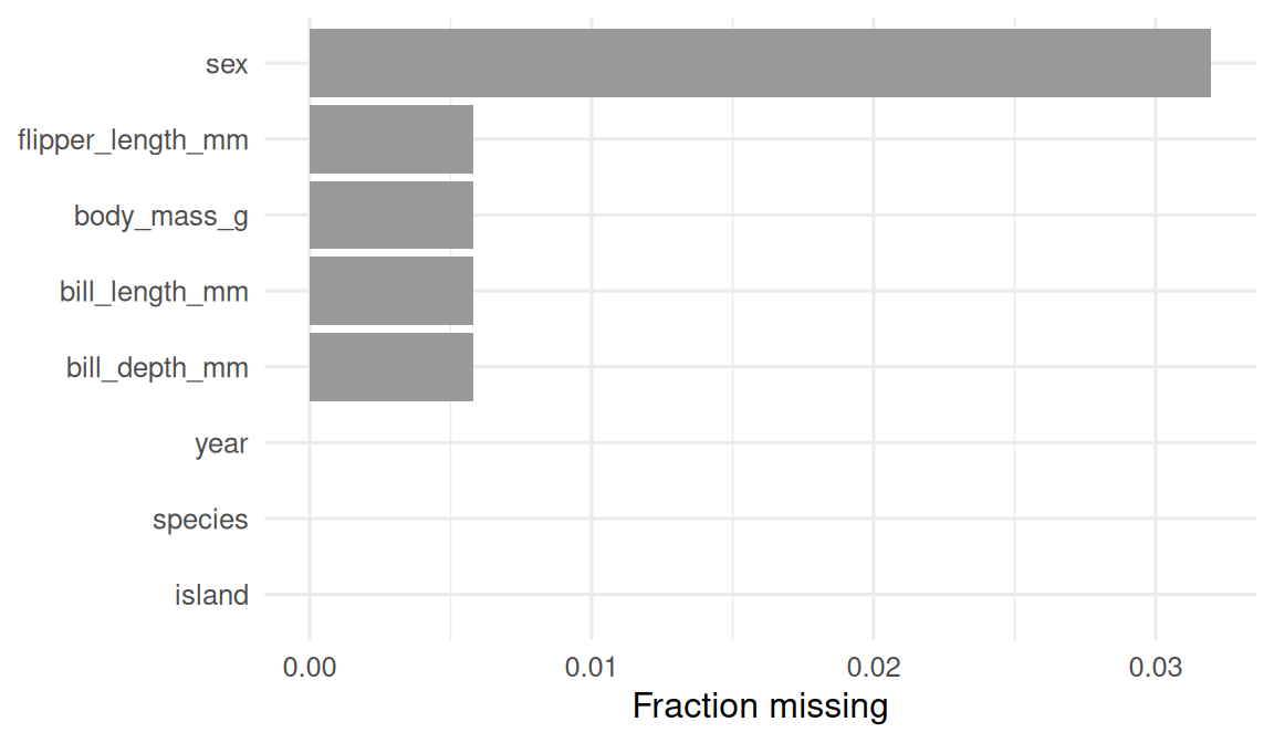

missingness |>
  ggplot(aes(frac_missing, reorder(variable, frac_missing))) +
  geom_col(fill = "grey60") +
  labs(x = "Fraction missing", y = NULL)

Now inject missingness to show how NAs move through a pipeline.

n <- nrow(penguins)
inj <- penguins |>
  mutate(body_mass_g = if_else(runif(n) < 0.1, NA_real_, body_mass_g))
mean(inj$body_mass_g)            # NA — propagates

[1] NA

mean(inj$body_mass_g, na.rm = TRUE)

[1] 4213.026

5. Report

Of the 344 rows in palmerpenguins::penguins, sex was missing in 11 rows (3.2%) and the four morphometric variables were missing in two rows apiece. After an inner join with a three-row islands table, all rows matched. Missingness was quantified per-variable and any summary that took a mean used na.rm = TRUE explicitly; silent NA propagation would otherwise have produced an NA mean.

Always look at the pattern of missingness before running an analysis. If NAs cluster in one group, a list-wise delete changes the comparison you thought you were making.

Common pitfalls

Forgetting na.rm = TRUE in a mean() and getting back an NA.
Confusing inner and left join and silently dropping rows.
Using row numbers as join keys after a reshape (they will not match).
Imputing missingness by hand and forgetting to flag the imputed rows.

Session info

sessionInfo()

R version 4.4.1 (2024-06-14)
Platform: x86_64-pc-linux-gnu
Running under: Ubuntu 24.04.4 LTS

Matrix products: default
BLAS:   /usr/lib/x86_64-linux-gnu/openblas-pthread/libblas.so.3 
LAPACK: /usr/lib/x86_64-linux-gnu/openblas-pthread/libopenblasp-r0.3.26.so;  LAPACK version 3.12.0

locale:
 [1] LC_CTYPE=C.UTF-8       LC_NUMERIC=C           LC_TIME=C.UTF-8       
 [4] LC_COLLATE=C.UTF-8     LC_MONETARY=C.UTF-8    LC_MESSAGES=C.UTF-8   
 [7] LC_PAPER=C.UTF-8       LC_NAME=C              LC_ADDRESS=C          
[10] LC_TELEPHONE=C         LC_MEASUREMENT=C.UTF-8 LC_IDENTIFICATION=C   

time zone: UTC
tzcode source: system (glibc)

attached base packages:
[1] stats     graphics  grDevices utils     datasets  methods   base     

other attached packages:
 [1] palmerpenguins_0.1.1 lubridate_1.9.5      forcats_1.0.1       
 [4] stringr_1.6.0        dplyr_1.2.1          purrr_1.2.2         
 [7] readr_2.2.0          tidyr_1.3.2          tibble_3.3.1        
[10] ggplot2_4.0.3        tidyverse_2.0.0     

loaded via a namespace (and not attached):
 [1] gtable_0.3.6       jsonlite_2.0.0     compiler_4.4.1     tidyselect_1.2.1  
 [5] scales_1.4.0       yaml_2.3.12        fastmap_1.2.0      R6_2.6.1          
 [9] labeling_0.4.3     generics_0.1.4     knitr_1.51         htmlwidgets_1.6.4 
[13] pillar_1.11.1      RColorBrewer_1.1-3 tzdb_0.5.0         rlang_1.2.0       
[17] utf8_1.2.6         stringi_1.8.7      xfun_0.57          S7_0.2.2          
[21] otel_0.2.0         timechange_0.4.0   cli_3.6.6          withr_3.0.2       
[25] magrittr_2.0.5     digest_0.6.39      grid_4.4.1         hms_1.1.4         
[29] lifecycle_1.0.5    vctrs_0.7.3        evaluate_1.0.5     glue_1.8.1        
[33] farver_2.1.2       rmarkdown_2.31     tools_4.4.1        pkgconfig_2.0.3   
[37] htmltools_0.5.9

Week 1, Session 4 — Import, joins, and missingness with dplyr

Learning objectives

Prerequisites

Background

Setup

1. Goal

2. Approach

3. Execution

4. Check

5. Report

Common pitfalls

Further reading

Session info