Week 2, Session 3 — Diagnostic testing: Se, Sp, PPV, NPV, LR

Course 1 — #courses

R. Heller

Note

Inference labs use the five-step template: Hypothesis → Visualise → Assumptions → Conduct → Conclude.

Learning objectives

• Compute sensitivity, specificity, PPV, NPV, and positive and negative likelihood ratios from a 2x2 table.
• Convert pre-test probability to post-test probability with an LR.
• Sketch a receiver-operating characteristic curve from a continuous test statistic.

Prerequisites

Lab 2.2.

Background

A diagnostic test has two operating characteristics intrinsic to the test itself: sensitivity is the probability that a diseased person tests positive; specificity is the probability that a disease-free person tests negative. These quantities are properties of the test. They do not change with prevalence.

Two other quantities are properties of the test and the population in which it is applied: positive predictive value is the probability of disease given a positive test; negative predictive value is the probability of no disease given a negative test. These change with prevalence, sometimes dramatically.

Likelihood ratios unify the two pairs. LR+ is sens / (1 − spec); LR− is (1 − sens) / spec. They convert pre-test odds to post-test odds by multiplication, which is the cleanest way to combine a test result with prior information. An LR+ greater than 10 is a strong positive; less than 0.1 is a strong negative; values near 1 are uninformative.

Setup

library(tidyverse)
set.seed(42)
theme_set(theme_minimal(base_size = 12))

1. Hypothesis

Question of interest: how does a continuous biomarker behave as a diagnostic test? We are not running an inferential test; we are characterising a test’s discrimination.

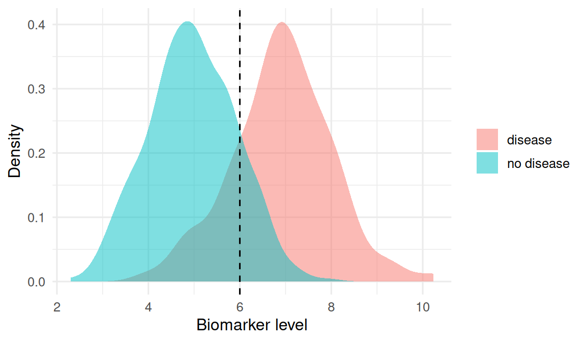
2. Visualise

Simulate a biomarker that is higher in diseased cases than in disease-free controls, with overlap.

N <- 500
prev <- 0.2
pop <- tibble(
  id = seq_len(N),
  disease = rbinom(N, 1, prev),
  biomarker = rnorm(N, mean = if_else(disease == 1, 7, 5), sd = 1)
)

pop |>
  mutate(status = if_else(disease == 1, "disease", "no disease")) |>
  ggplot(aes(biomarker, fill = status)) +
  geom_density(alpha = 0.5, colour = NA) +
  geom_vline(xintercept = 6, linetype = 2) +
  labs(x = "Biomarker level", y = "Density", fill = NULL)

3. Assumptions

The gold standard for disease status is assumed perfect. The biomarker is continuous and must be dichotomised at some cutoff to behave like a positive/negative test. We choose 6 as the cutoff for illustration; in practice, the cutoff is itself an outcome of the analysis.

cutoff <- 6
pop <- pop |> mutate(test = as.integer(biomarker > cutoff))
tab <- table(disease = pop$disease, test = pop$test)
tab

       test
disease   0   1
      0 346  53
      1  21  80

4. Conduct

TP <- tab["1", "1"]; FN <- tab["1", "0"]
FP <- tab["0", "1"]; TN <- tab["0", "0"]

sens <- TP / (TP + FN)
spec <- TN / (TN + FP)
ppv  <- TP / (TP + FP)
npv  <- TN / (TN + FN)
lrp  <- sens / (1 - spec)
lrn  <- (1 - sens) / spec

diag_tbl <- tibble(
  quantity = c("Sensitivity", "Specificity",
               "PPV", "NPV", "LR+", "LR-"),
  value = c(sens, spec, ppv, npv, lrp, lrn)
)
diag_tbl

# A tibble: 6 × 2
  quantity    value
  <chr>       <dbl>
1 Sensitivity 0.792
2 Specificity 0.867
3 PPV         0.602
4 NPV         0.943
5 LR+         5.96 
6 LR-         0.240

Convert pre-test odds to post-test odds with the LR.

pre_prob <- 0.1
pre_odds <- pre_prob / (1 - pre_prob)
post_odds_pos <- pre_odds * lrp
post_prob_pos <- post_odds_pos / (1 + post_odds_pos)
post_odds_neg <- pre_odds * lrn
post_prob_neg <- post_odds_neg / (1 + post_odds_neg)

tibble(
  pre_prob,
  post_prob_if_positive = post_prob_pos,
  post_prob_if_negative = post_prob_neg
)

# A tibble: 1 × 3
  pre_prob post_prob_if_positive post_prob_if_negative
     <dbl>                 <dbl>                 <dbl>
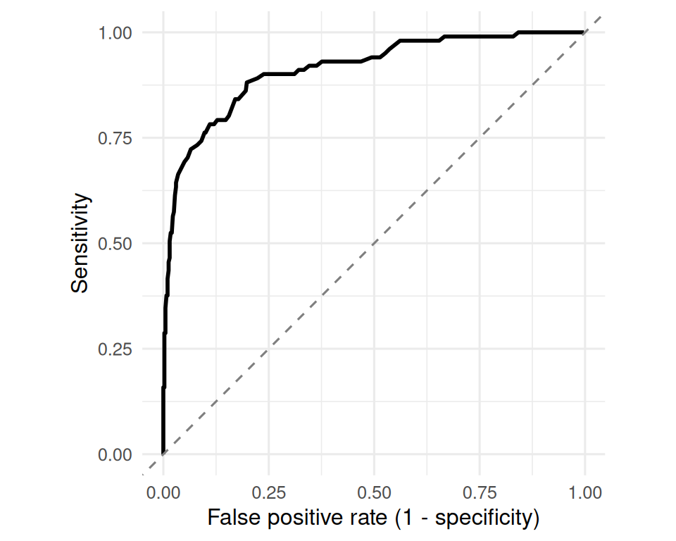
1      0.1                 0.399                0.0259

Sketch an ROC by sweeping the cutoff.

roc <- tibble(
  cut = seq(min(pop$biomarker), max(pop$biomarker), length.out = 200)
) |>
  rowwise() |>
  mutate(
    tp = sum(pop$biomarker > cut & pop$disease == 1),
    fn = sum(pop$biomarker <= cut & pop$disease == 1),
    fp = sum(pop$biomarker > cut & pop$disease == 0),
    tn = sum(pop$biomarker <= cut & pop$disease == 0),
    sens = tp / (tp + fn),
    fpr  = fp / (fp + tn)
  ) |>
  ungroup()

ggplot(roc, aes(fpr, sens)) +
  geom_path(linewidth = 1) +
  geom_abline(linetype = 2, colour = "grey50") +
  coord_equal() +
  labs(x = "False positive rate (1 - specificity)",
       y = "Sensitivity")

5. Concluding statement

With a cutoff of 6, the biomarker had sensitivity 0.79, specificity 0.87, PPV 0.6, and NPV 0.94. The positive likelihood ratio was 5.96 and the negative 0.24. A pre-test probability of 10% becomes 0.4 after a positive test and 0.026 after a negative test.

A single cutoff collapses a rich continuous score into two states. The ROC curve shows the trade-off across all cutoffs; the area under it summarises overall discrimination without committing to a threshold.

Walk through the ROC construction cut-by-cut. Emphasise that no point on the curve is the “right” one — the right one depends on the relative cost of a false positive vs. a false negative.

Common pitfalls

• Quoting a single cutoff’s sensitivity and specificity as if they were fixed properties of the test, ignoring that a different cutoff gives different numbers.
• Confusing sensitivity with PPV in everyday speech.
• Forgetting that PPV and NPV depend on prevalence.
• Using an ROC to compare tests with different prevalence in each sample.

Further reading

• Altman DG & Bland JM, Diagnostic tests series, BMJ.
• Pepe MS. The Statistical Evaluation of Medical Tests for Classification and Prediction.

Session info

sessionInfo()

R version 4.4.1 (2024-06-14)
Platform: x86_64-pc-linux-gnu
Running under: Ubuntu 24.04.4 LTS

Matrix products: default
BLAS:   /usr/lib/x86_64-linux-gnu/openblas-pthread/libblas.so.3 
LAPACK: /usr/lib/x86_64-linux-gnu/openblas-pthread/libopenblasp-r0.3.26.so;  LAPACK version 3.12.0

locale:
 [1] LC_CTYPE=C.UTF-8       LC_NUMERIC=C           LC_TIME=C.UTF-8       
 [4] LC_COLLATE=C.UTF-8     LC_MONETARY=C.UTF-8    LC_MESSAGES=C.UTF-8   
 [7] LC_PAPER=C.UTF-8       LC_NAME=C              LC_ADDRESS=C          
[10] LC_TELEPHONE=C         LC_MEASUREMENT=C.UTF-8 LC_IDENTIFICATION=C   

time zone: UTC
tzcode source: system (glibc)

attached base packages:
[1] stats     graphics  grDevices utils     datasets  methods   base     

other attached packages:
 [1] lubridate_1.9.5 forcats_1.0.1   stringr_1.6.0   dplyr_1.2.1    
 [5] purrr_1.2.2     readr_2.2.0     tidyr_1.3.2     tibble_3.3.1   
 [9] ggplot2_4.0.3   tidyverse_2.0.0

loaded via a namespace (and not attached):
 [1] gtable_0.3.6       jsonlite_2.0.0     compiler_4.4.1     tidyselect_1.2.1  
 [5] scales_1.4.0       yaml_2.3.12        fastmap_1.2.0      R6_2.6.1          
 [9] labeling_0.4.3     generics_0.1.4     knitr_1.51         htmlwidgets_1.6.4 
[13] pillar_1.11.1      RColorBrewer_1.1-3 tzdb_0.5.0         rlang_1.2.0       
[17] utf8_1.2.6         stringi_1.8.7      xfun_0.57          S7_0.2.2          
[21] otel_0.2.0         timechange_0.4.0   cli_3.6.6          withr_3.0.2       
[25] magrittr_2.0.5     digest_0.6.39      grid_4.4.1         hms_1.1.4         
[29] lifecycle_1.0.5    vctrs_0.7.3        evaluate_1.0.5     glue_1.8.1        
[33] farver_2.1.2       rmarkdown_2.31     tools_4.4.1        pkgconfig_2.0.3   
[37] htmltools_0.5.9