Week 2, Session 4 — Discrete distributions: Bernoulli, binomial, Poisson

Course 1 — #courses

R. Heller

Note

Inference labs use the five-step template: Hypothesis → Visualise → Assumptions → Conduct → Conclude.

Learning objectives

• Simulate Bernoulli trials and aggregate them to a binomial.
• Show the Poisson approximation to the binomial when n is large and p is small.
• Use dbinom(), pbinom(), and rbinom() (and their Poisson counterparts) to answer probability questions.

Prerequisites

Lab 2.2 (probability).

Background

The Bernoulli distribution is the simplest non-trivial distribution: one coin, two outcomes, a single probability p. The binomial adds structure — n independent Bernoulli trials with the same p — and gives the distribution of the count of successes. The Poisson arises in the limit where n is large, p is small, and np stays fixed; it describes counts of rare events over a fixed window of opportunity, without needing to specify n and p separately.

Most count-like quantities in biomedicine can be modelled by one of these three. Whether a tumour is responding (Bernoulli), how many of twenty patients relapse (binomial), how many emergency admissions arrive in an hour (Poisson) — the same three distributions cover a great deal of ground. The simulation-first approach makes them concrete before we write a formula.

There is a common conflation between the binomial and the Poisson in the clinical literature. When the sample size is large and the event is rare, the two distributions give nearly identical probabilities and either is defensible. When the event is not rare, the Poisson can assign meaningful probability to impossible events (more successes than trials), so the binomial is strictly better.

Setup

library(tidyverse)
set.seed(42)
theme_set(theme_minimal(base_size = 12))

1. Hypothesis

We characterise three discrete distributions by simulation, then compare the empirical frequencies to the theoretical probabilities. No hypothesis is tested.

2. Visualise

A Bernoulli trial: one coin, success probability 0.3.

n_trials <- 1000
bern <- rbinom(n_trials, 1, 0.3)
mean(bern)   # empirical p

[1] 0.293

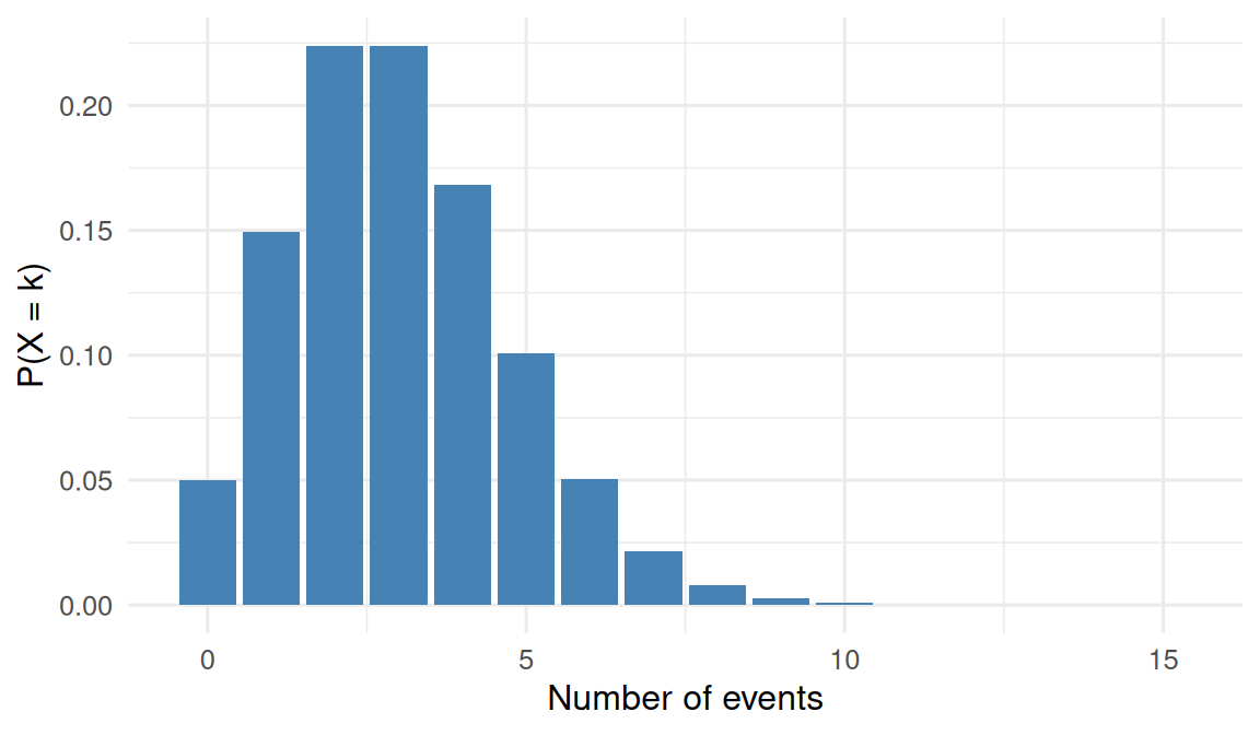
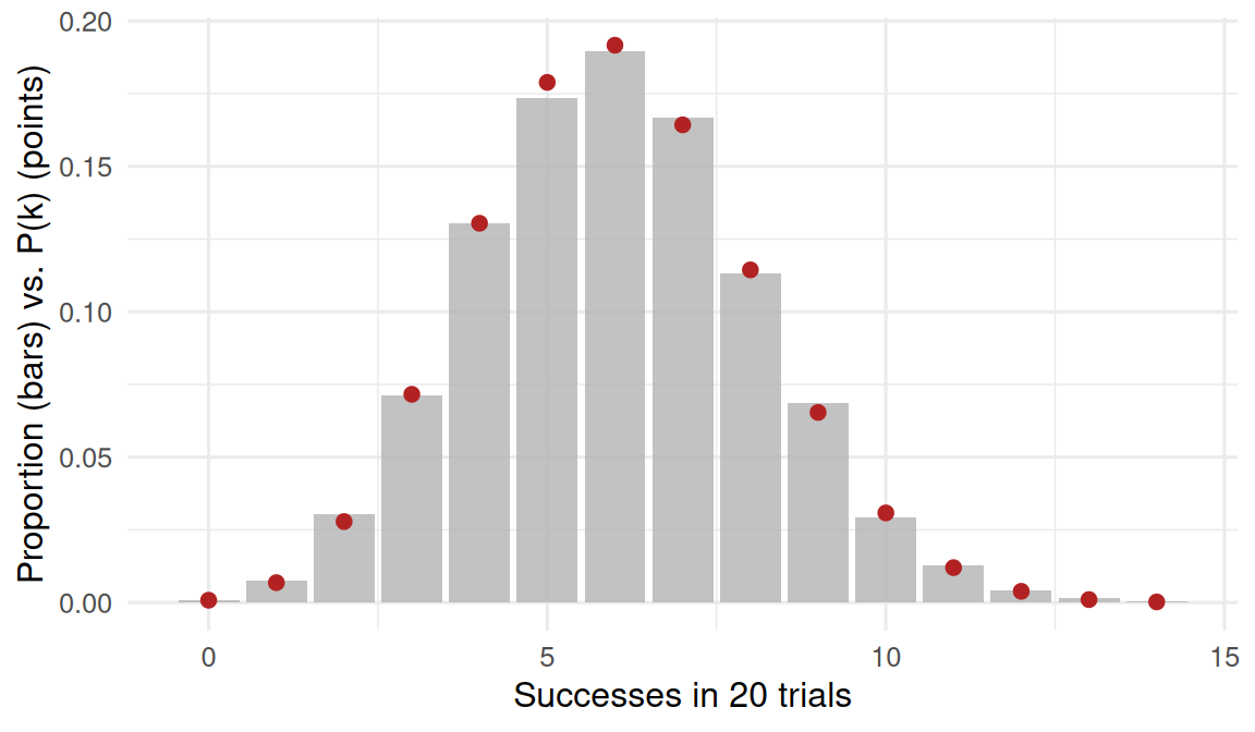
A binomial count: how many successes in 20 trials each at p = 0.3, repeated 10,000 times.

n_rep <- 10000
bin  <- rbinom(n_rep, size = 20, prob = 0.3)

bin_tibble <- tibble(k = bin) |>
  count(k) |>
  mutate(prop = n / sum(n),
         theo = dbinom(k, 20, 0.3))

bin_tibble |>
  ggplot(aes(k, prop)) +
  geom_col(fill = "grey70", alpha = 0.8) +
  geom_point(aes(y = theo), colour = "firebrick", size = 2) +
  labs(x = "Successes in 20 trials",
       y = "Proportion (bars) vs. P(k) (points)")

3. Assumptions

Binomial assumes fixed n, independence, and constant p. Poisson assumes a constant rate and independent counts over disjoint intervals. When n is large and p is small with np = λ, the binomial approaches Poisson.

# n=1000, p=0.003, so np = 3. Compare binomial and Poisson probabilities.
probs <- tibble(
  k = 0:10,
  binom  = dbinom(k, 1000, 0.003),
  pois   = dpois(k, 3)
)
probs

# A tibble: 11 × 3
       k    binom     pois
   <int>    <dbl>    <dbl>
 1     0 0.0496   0.0498  
 2     1 0.149    0.149   
 3     2 0.224    0.224   
 4     3 0.224    0.224   
 5     4 0.168    0.168   
 6     5 0.101    0.101   
 7     6 0.0503   0.0504  
 8     7 0.0215   0.0216  
 9     8 0.00803  0.00810 
10     9 0.00266  0.00270 
11    10 0.000794 0.000810

4. Conduct

Answer two specific questions.

# Q1: In a trial of 20 patients at p=0.3 response rate, what is
# P(at least 8 responders)?
p_ge8 <- 1 - pbinom(7, size = 20, prob = 0.3)
p_ge8

[1] 0.2277282

# Q2: An ER admits patients at a rate of 3/hour. What is
# P(7 or more patients in a given hour)?
p_pois_ge7 <- 1 - ppois(6, lambda = 3)
p_pois_ge7

[1] 0.03350854

Simulate Q2 to confirm.

sim <- rpois(10000, lambda = 3)
mean(sim >= 7)

[1] 0.0354

tibble(k = 0:15) |>
  mutate(pois_density = dpois(k, 3)) |>
  ggplot(aes(k, pois_density)) +
  geom_col(fill = "steelblue") +
  labs(x = "Number of events", y = "P(X = k)")

5. Concluding statement

A response rate of 0.3 in a 20-patient trial implies a probability of 0.228 of observing eight or more responders. An ER with a mean admission rate of 3/hour has a probability of 0.034 of receiving seven or more admissions in a given hour; 10,000 simulated hours recovered an empirical proportion of 0.035. The binomial with n = 1000, p = 0.003 and the Poisson with λ = 3 gave nearly indistinguishable probabilities across k = 0–10.

Discrete distributions are under-appreciated. Many designs that are reached for as continuous (eg regressions on a rate) have a cleaner count-based model sitting next to them.

Make the binomial → Poisson limit visible: plot the two PMFs on the same axes at decreasing p and watch them converge.

Common pitfalls

• Using the normal approximation to the binomial when n is small. For small n use pbinom() directly.
• Modelling a rate as a proportion when the denominator is person-time, not persons.
• Treating a Poisson with a known λ as if its variance had to be estimated. For Poisson, mean = variance.

Further reading

• Rosner B. Fundamentals of Biostatistics, chapter on discrete distributions.
• Agresti A. Categorical Data Analysis, opening chapter.

Session info

sessionInfo()

R version 4.4.1 (2024-06-14)
Platform: x86_64-pc-linux-gnu
Running under: Ubuntu 24.04.4 LTS

Matrix products: default
BLAS:   /usr/lib/x86_64-linux-gnu/openblas-pthread/libblas.so.3 
LAPACK: /usr/lib/x86_64-linux-gnu/openblas-pthread/libopenblasp-r0.3.26.so;  LAPACK version 3.12.0

locale:
 [1] LC_CTYPE=C.UTF-8       LC_NUMERIC=C           LC_TIME=C.UTF-8       
 [4] LC_COLLATE=C.UTF-8     LC_MONETARY=C.UTF-8    LC_MESSAGES=C.UTF-8   
 [7] LC_PAPER=C.UTF-8       LC_NAME=C              LC_ADDRESS=C          
[10] LC_TELEPHONE=C         LC_MEASUREMENT=C.UTF-8 LC_IDENTIFICATION=C   

time zone: UTC
tzcode source: system (glibc)

attached base packages:
[1] stats     graphics  grDevices utils     datasets  methods   base     

other attached packages:
 [1] lubridate_1.9.5 forcats_1.0.1   stringr_1.6.0   dplyr_1.2.1    
 [5] purrr_1.2.2     readr_2.2.0     tidyr_1.3.2     tibble_3.3.1   
 [9] ggplot2_4.0.3   tidyverse_2.0.0

loaded via a namespace (and not attached):
 [1] gtable_0.3.6       jsonlite_2.0.0     compiler_4.4.1     tidyselect_1.2.1  
 [5] scales_1.4.0       yaml_2.3.12        fastmap_1.2.0      R6_2.6.1          
 [9] labeling_0.4.3     generics_0.1.4     knitr_1.51         htmlwidgets_1.6.4 
[13] pillar_1.11.1      RColorBrewer_1.1-3 tzdb_0.5.0         rlang_1.2.0       
[17] stringi_1.8.7      xfun_0.57          S7_0.2.2           otel_0.2.0        
[21] timechange_0.4.0   cli_3.6.6          withr_3.0.2        magrittr_2.0.5    
[25] digest_0.6.39      grid_4.4.1         hms_1.1.4          lifecycle_1.0.5   
[29] vctrs_0.7.3        evaluate_1.0.5     glue_1.8.1         farver_2.1.2      
[33] rmarkdown_2.31     tools_4.4.1        pkgconfig_2.0.3    htmltools_0.5.9