Week 2, Session 5 — Continuous distributions and Q-Q plots

Course 1 — #courses

R. Heller

Note

Inference labs use the five-step template: Hypothesis → Visualise → Assumptions → Conduct → Conclude.

Learning objectives

• Draw densities of the normal, t, chi-square, F, and exponential distributions and describe how shape changes with parameters.
• Use Q-Q plots to assess whether data are consistent with a hypothesised distribution.
• Recognise the degrees-of-freedom relationships among the normal-derived distributions.

Prerequisites

Lab 2.4.

Background

The continuous distributions in this lab cover the majority of routine parametric inference. The normal is the distribution of means under the central limit theorem. The t is what happens to the normal when the variance is itself estimated from the data — with more uncertainty (smaller n), heavier tails. The chi-square is the distribution of sums of squared standard normals. The F is a ratio of chi-squares. The exponential appears in survival and queueing.

The Q-Q plot is the workhorse for assessing distributional fit. Plotting sample quantiles against theoretical quantiles gives a straight line when the model is right. Deviations at the tails indicate skew or heavy tails; an S-shape indicates non-normal symmetric behaviour. Q-Q plots are how assumptions of the t-test and the analysis of variance get checked in practice.

Degrees of freedom are easy to mis-remember. The short version: t has df = n − 1 for a one-sample test; chi-square from a sum of k squared standard normals has df = k; F has two df — numerator and denominator — that come from the chi-squares in its ratio.

Setup

library(tidyverse)
set.seed(42)
theme_set(theme_minimal(base_size = 12))

1. Hypothesis

We are not testing a hypothesis. We are characterising five continuous distributions and using Q-Q plots to assess whether a sample is consistent with a model.

2. Visualise

Plot densities side by side.

grid <- tibble(x = seq(-5, 5, length.out = 400))

densities <- bind_rows(
  grid |> mutate(density = dnorm(x),         dist = "Normal(0,1)"),
  grid |> mutate(density = dt(x, df = 3),    dist = "t(3)"),
  grid |> mutate(density = dt(x, df = 30),   dist = "t(30)")
)

ggplot(densities, aes(x, density, colour = dist)) +
  geom_line(linewidth = 1) +
  labs(x = NULL, y = "Density", colour = NULL)

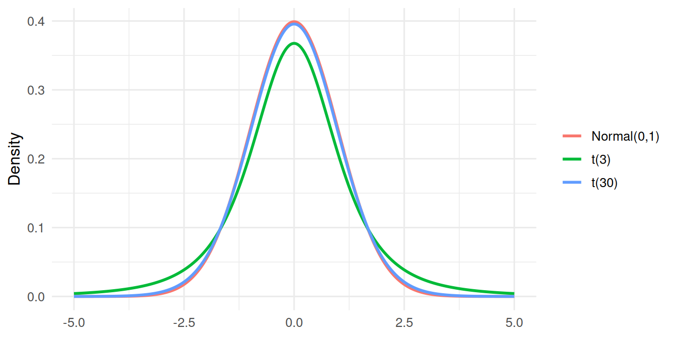
The t with 3 df has visibly heavier tails; at 30 df it is nearly normal.

chi_grid <- tibble(x = seq(0.01, 20, length.out = 400))
chi <- bind_rows(
  chi_grid |> mutate(density = dchisq(x, df = 2), dist = "chi-sq(2)"),
  chi_grid |> mutate(density = dchisq(x, df = 5), dist = "chi-sq(5)"),
  chi_grid |> mutate(density = dchisq(x, df = 10), dist = "chi-sq(10)")
)

ggplot(chi, aes(x, density, colour = dist)) +
  geom_line(linewidth = 1) +
  labs(x = NULL, y = "Density", colour = NULL)

3. Assumptions

We assume samples are independent and identically distributed. For the Q-Q check, the sample must be reasonably sized (say, at least 20 observations) for the plot to be informative.

# Facet across df for the F distribution.
f_grid <- expand_grid(
  x  = seq(0.01, 5, length.out = 300),
  df1 = c(2, 5, 10),
  df2 = c(10, 30)
) |>
  mutate(density = df(x, df1, df2))

f_grid |>
  ggplot(aes(x, density, colour = factor(df1))) +
  geom_line(linewidth = 1) +
  facet_wrap(~ df2, labeller = label_both) +
  labs(x = NULL, y = "Density", colour = "df1")

4. Conduct

Q-Q plots. Simulate data, compare to a hypothesised distribution.

n <- 200
samples <- tibble(
  normal_sample = rnorm(n),
  heavy_tail    = rt(n, df = 3),
  exponential   = rexp(n, rate = 1)
)

samples |>
  pivot_longer(everything(), names_to = "sample", values_to = "value") |>
  ggplot(aes(sample = value)) +
  stat_qq(alpha = 0.6) +
  stat_qq_line(colour = "firebrick") +
  facet_wrap(~ sample, scales = "free") +
  labs(x = "Theoretical normal quantiles",
       y = "Sample quantiles")

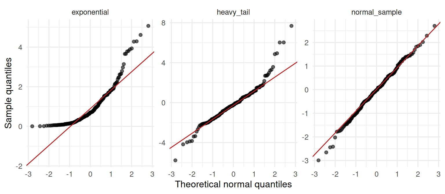
The normal sample lies on the 45° reference line; the heavy-tailed sample splays at both ends; the exponential curves away on one side.

Shapiro-Wilk as a quick numerical check on the three samples.

sw_results <- samples |>
  pivot_longer(everything(), names_to = "sample", values_to = "value") |>
  group_by(sample) |>
  summarise(p = shapiro.test(value)$p.value, .groups = "drop")
sw_results

# A tibble: 3 × 2
  sample               p
  <chr>            <dbl>
1 exponential   3.74e-14
2 heavy_tail    3.42e- 7
3 normal_sample 9.46e- 1

5. Concluding statement

The normal sample (n = 200) was consistent with normality both visually (Q-Q line) and by Shapiro-Wilk (p = 0.95). The t(3) sample showed clear tail departures, Shapiro-Wilk p = 3.4^{-7}. The exponential sample was strongly right-skewed, p < 0.001.

A Q-Q plot is the most information-dense way to inspect a distributional assumption. Numerical tests of normality (Shapiro-Wilk, Kolmogorov-Smirnov) should corroborate, not replace, the plot.

Insist on the plot. Large samples will flag any small deviation as significant on Shapiro-Wilk; small samples will find nothing significant even when the distribution is wrong.

Common pitfalls

• Reading the centre of a Q-Q plot and ignoring the tails. The tails are where the interesting departures live.
• Declaring a distribution wrong on Shapiro-Wilk in a sample of 5000 when the Q-Q plot is straight.
• Forgetting that t approaches normal as df → ∞; do not test with df = 500 in a fit-diagnostic mindset.

Further reading

• Rice JA. Mathematical Statistics and Data Analysis.
• Kutner MH et al. Applied Linear Statistical Models.

Session info

sessionInfo()

R version 4.4.1 (2024-06-14)
Platform: x86_64-pc-linux-gnu
Running under: Ubuntu 24.04.4 LTS

Matrix products: default
BLAS:   /usr/lib/x86_64-linux-gnu/openblas-pthread/libblas.so.3 
LAPACK: /usr/lib/x86_64-linux-gnu/openblas-pthread/libopenblasp-r0.3.26.so;  LAPACK version 3.12.0

locale:
 [1] LC_CTYPE=C.UTF-8       LC_NUMERIC=C           LC_TIME=C.UTF-8       
 [4] LC_COLLATE=C.UTF-8     LC_MONETARY=C.UTF-8    LC_MESSAGES=C.UTF-8   
 [7] LC_PAPER=C.UTF-8       LC_NAME=C              LC_ADDRESS=C          
[10] LC_TELEPHONE=C         LC_MEASUREMENT=C.UTF-8 LC_IDENTIFICATION=C   

time zone: UTC
tzcode source: system (glibc)

attached base packages:
[1] stats     graphics  grDevices utils     datasets  methods   base     

other attached packages:
 [1] lubridate_1.9.5 forcats_1.0.1   stringr_1.6.0   dplyr_1.2.1    
 [5] purrr_1.2.2     readr_2.2.0     tidyr_1.3.2     tibble_3.3.1   
 [9] ggplot2_4.0.3   tidyverse_2.0.0

loaded via a namespace (and not attached):
 [1] gtable_0.3.6       jsonlite_2.0.0     compiler_4.4.1     tidyselect_1.2.1  
 [5] scales_1.4.0       yaml_2.3.12        fastmap_1.2.0      R6_2.6.1          
 [9] labeling_0.4.3     generics_0.1.4     knitr_1.51         htmlwidgets_1.6.4 
[13] pillar_1.11.1      RColorBrewer_1.1-3 tzdb_0.5.0         rlang_1.2.0       
[17] utf8_1.2.6         stringi_1.8.7      xfun_0.57          S7_0.2.2          
[21] otel_0.2.0         timechange_0.4.0   cli_3.6.6          withr_3.0.2       
[25] magrittr_2.0.5     digest_0.6.39      grid_4.4.1         hms_1.1.4         
[29] lifecycle_1.0.5    vctrs_0.7.3        evaluate_1.0.5     glue_1.8.1        
[33] farver_2.1.2       rmarkdown_2.31     tools_4.4.1        pkgconfig_2.0.3   
[37] htmltools_0.5.9