Week 3, Session 2 — Bootstrap and permutation tests

Course 1 — #courses

R. Heller

Note

Inference labs use the five-step template: Hypothesis → Visualise → Assumptions → Conduct → Conclude.

Learning objectives

• Compute a bootstrap confidence interval for a statistic whose sampling distribution is not easily derived.
• Run a permutation test for a two-group comparison and state what null hypothesis it tests.
• Explain when bootstrap and permutation answer different questions.

Prerequisites

Lab 3.1.

Background

Classical inference writes down the sampling distribution of an estimator analytically, usually by invoking the central limit theorem and assuming a parametric family for the data. Resampling methods replace this step with computation. A bootstrap confidence interval for a statistic is built by drawing repeated samples with replacement from the observed data and recomputing the statistic; the empirical distribution of the recomputed values is treated as a proxy for the sampling distribution.

A permutation test answers a different question. It randomly reassigns the group labels on the observed data and recomputes the test statistic; the empirical distribution of the recomputed values is the sampling distribution under the null of exchangeability — that is, under a null in which the group labels are interchangeable. It gives a p-value without any assumption about the shape of the underlying distributions.

The two techniques look similar — both involve a loop and a replicate() — but they are different tools. Bootstrap estimates uncertainty under the observed data-generating process; permutation tests a sharp null of no association.

Setup

library(tidyverse)
set.seed(42)
theme_set(theme_minimal(base_size = 12))

1. Hypothesis

Two hypotheses in this lab:

1. For a sample median of body mass in Gentoo penguins, build a 95% bootstrap CI.
2. For flipper length in Gentoo vs Adelie penguins, test the sharp null that the distributions are exchangeable against the two-sided alternative.

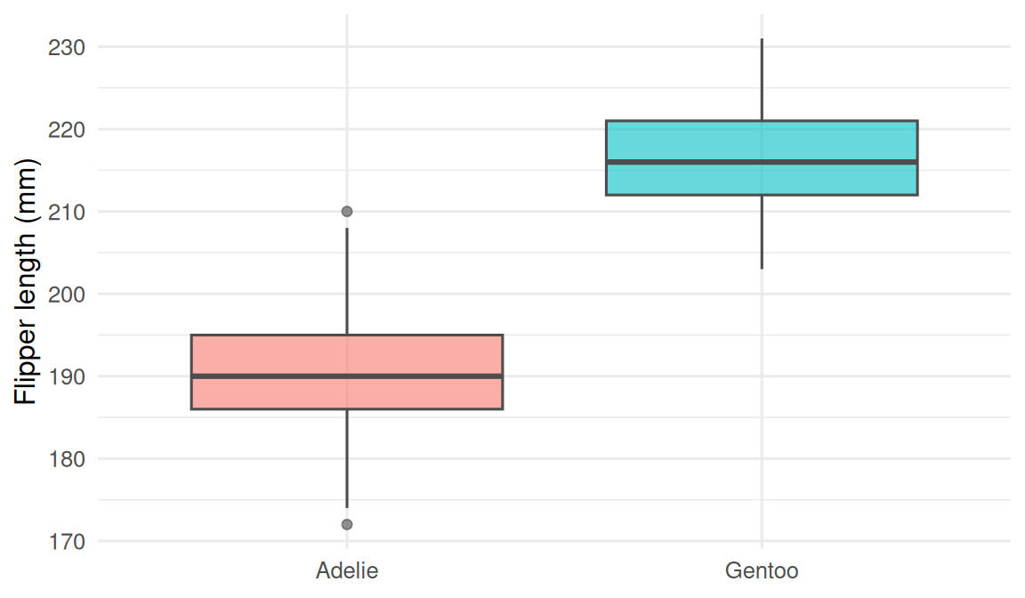
2. Visualise

Use palmerpenguins.

library(palmerpenguins)
dat <- penguins |>
  filter(species %in% c("Gentoo", "Adelie")) |>
  drop_na(body_mass_g, flipper_length_mm)

dat |>
  ggplot(aes(species, flipper_length_mm, fill = species)) +
  geom_boxplot(alpha = 0.6, colour = "grey30") +
  labs(x = NULL, y = "Flipper length (mm)") +
  theme(legend.position = "none")

3. Assumptions

Bootstrap: the observed sample is representative of the population we wish to generalise to. Resampling with replacement preserves the univariate structure but assumes exchangeability of observations.

Permutation: under H0, group labels can be reshuffled without changing the joint distribution. The test does not assume normality or equal variances.

4. Conduct

Bootstrap CI for the median body mass of Gentoo

gen <- dat |> filter(species == "Gentoo") |> pull(body_mass_g)
B <- 2000
boot_meds <- replicate(B, median(sample(gen, replace = TRUE)))
ci_med <- quantile(boot_meds, c(0.025, 0.975))
obs_med <- median(gen)
tibble(statistic = "median body mass",
       observed = obs_med,
       ci_low = ci_med[1],
       ci_high = ci_med[2])

# A tibble: 1 × 4
  statistic        observed ci_low ci_high
  <chr>               <int>  <dbl>   <dbl>
1 median body mass     5000   4900    5200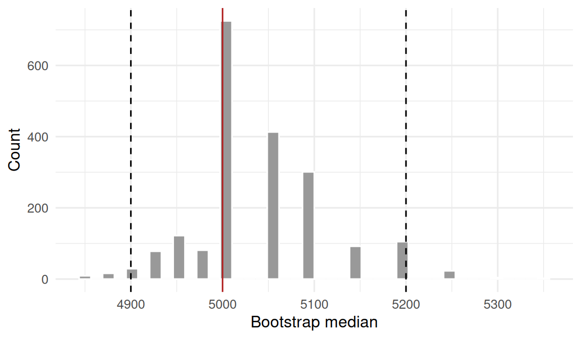

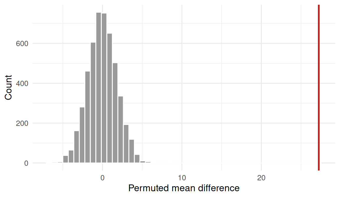
tibble(boot = boot_meds) |>
  ggplot(aes(boot)) +
  geom_histogram(bins = 40, fill = "grey60", colour = "white") +
  geom_vline(xintercept = obs_med, colour = "firebrick") +
  geom_vline(xintercept = ci_med, linetype = 2) +
  labs(x = "Bootstrap median", y = "Count")

Permutation test for flipper length Gentoo vs Adelie

g <- dat$species
x <- dat$flipper_length_mm
observed_diff <- mean(x[g == "Gentoo"]) - mean(x[g == "Adelie"])

perm_diff <- replicate(5000, {
  gp <- sample(g)
  mean(x[gp == "Gentoo"]) - mean(x[gp == "Adelie"])
})
p_perm <- mean(abs(perm_diff) >= abs(observed_diff))
p_perm

[1] 0

tibble(perm = perm_diff) |>
  ggplot(aes(perm)) +
  geom_histogram(bins = 50, fill = "grey60", colour = "white") +
  geom_vline(xintercept = observed_diff, colour = "firebrick", linewidth = 1) +
  labs(x = "Permuted mean difference", y = "Count")

5. Concluding statement

Based on B = 2000 bootstrap resamples, the median body mass in Gentoo penguins (n = 123) was 5000 g (95% percentile bootstrap CI 4900 to 5200 g). Flipper length was much longer in Gentoo than Adelie (mean difference 27.2 mm); a permutation test over 5000 reshuffles produced p = 0, providing strong evidence against exchangeability.

Bootstrap and permutation give you parametric-free tools for estimation and testing respectively. Neither rescues you from a biased sample; both depend on the data at hand being representative.

Emphasise the difference in what each method does: bootstrap = CI for the observed sampling regime; permutation = test of a sharp null. They do not compete.

Common pitfalls

• Using bootstrap SEs for a statistic with heavy tails (eg the maximum) — it does not have a well-defined bootstrap distribution.
• Permutation with more than two groups: you still need a single test statistic (eg F), not pairwise comparisons by default.
• Reading a bootstrap CI as a confidence interval for the population parameter when the sample is biased.

Further reading

• Efron B, Tibshirani RJ. An Introduction to the Bootstrap.
• Good PI. Permutation, Parametric, and Bootstrap Tests of Hypotheses.

Session info

sessionInfo()

R version 4.4.1 (2024-06-14)
Platform: x86_64-pc-linux-gnu
Running under: Ubuntu 24.04.4 LTS

Matrix products: default
BLAS:   /usr/lib/x86_64-linux-gnu/openblas-pthread/libblas.so.3 
LAPACK: /usr/lib/x86_64-linux-gnu/openblas-pthread/libopenblasp-r0.3.26.so;  LAPACK version 3.12.0

locale:
 [1] LC_CTYPE=C.UTF-8       LC_NUMERIC=C           LC_TIME=C.UTF-8       
 [4] LC_COLLATE=C.UTF-8     LC_MONETARY=C.UTF-8    LC_MESSAGES=C.UTF-8   
 [7] LC_PAPER=C.UTF-8       LC_NAME=C              LC_ADDRESS=C          
[10] LC_TELEPHONE=C         LC_MEASUREMENT=C.UTF-8 LC_IDENTIFICATION=C   

time zone: UTC
tzcode source: system (glibc)

attached base packages:
[1] stats     graphics  grDevices utils     datasets  methods   base     

other attached packages:
 [1] palmerpenguins_0.1.1 lubridate_1.9.5      forcats_1.0.1       
 [4] stringr_1.6.0        dplyr_1.2.1          purrr_1.2.2         
 [7] readr_2.2.0          tidyr_1.3.2          tibble_3.3.1        
[10] ggplot2_4.0.3        tidyverse_2.0.0     

loaded via a namespace (and not attached):
 [1] gtable_0.3.6       jsonlite_2.0.0     compiler_4.4.1     tidyselect_1.2.1  
 [5] scales_1.4.0       yaml_2.3.12        fastmap_1.2.0      R6_2.6.1          
 [9] labeling_0.4.3     generics_0.1.4     knitr_1.51         htmlwidgets_1.6.4 
[13] pillar_1.11.1      RColorBrewer_1.1-3 tzdb_0.5.0         rlang_1.2.0       
[17] utf8_1.2.6         stringi_1.8.7      xfun_0.57          S7_0.2.2          
[21] otel_0.2.0         timechange_0.4.0   cli_3.6.6          withr_3.0.2       
[25] magrittr_2.0.5     digest_0.6.39      grid_4.4.1         hms_1.1.4         
[29] lifecycle_1.0.5    vctrs_0.7.3        evaluate_1.0.5     glue_1.8.1        
[33] farver_2.1.2       rmarkdown_2.31     tools_4.4.1        pkgconfig_2.0.3   
[37] htmltools_0.5.9