Week 3, Session 3 — Maximum likelihood estimation

Course 1 — #courses

R. Heller

Note

Inference labs use the five-step template: Hypothesis → Visualise → Assumptions → Conduct → Conclude.

Learning objectives

• Write a log-likelihood for a simple model and find its maximum.
• Use Fisher information to obtain an asymptotic standard error and confidence interval.
• Relate the MLE to intuitive estimators (sample mean, sample rate).

Prerequisites

Lab 3.1.

Background

Maximum likelihood is the workhorse of parametric inference. Given a parametric family for the data — normal, Poisson, binomial — the MLE is the parameter value that makes the observed data most probable. Under mild regularity conditions the MLE is consistent (it converges to the truth), asymptotically unbiased, and asymptotically normal with variance given by the inverse of Fisher information.

Fisher information quantifies how sharply the log-likelihood peaks at its maximum. A sharply peaked likelihood gives a precise estimate (small variance); a flat one gives a vague estimate. The standard error of an MLE is the square root of 1/n times the inverse of the Fisher information per observation.

In the simple cases we treat here the MLE coincides with the intuitive estimator — the mean for a normal, the sample rate for a Poisson — but the machinery generalises to any likelihood.

Setup

library(tidyverse)
set.seed(42)
theme_set(theme_minimal(base_size = 12))

1. Hypothesis

Estimate (i) the mean of a normal and (ii) the rate of a Poisson by maximum likelihood, recover standard errors from Fisher information, and build Wald confidence intervals.

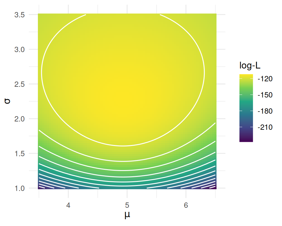
2. Visualise

Normal data with known σ = 2.

n <- 50
mu_true <- 5
sigma <- 2
x <- rnorm(n, mean = mu_true, sd = sigma)

grid <- tibble(mu = seq(3.5, 6.5, length.out = 300)) |>
  mutate(loglik = sapply(mu, function(m) sum(dnorm(x, m, sigma, log = TRUE))))
ggplot(grid, aes(mu, loglik)) +
  geom_line() +
  geom_vline(xintercept = mean(x), linetype = 2, colour = "firebrick") +
  labs(x = expression(mu), y = "log-likelihood")

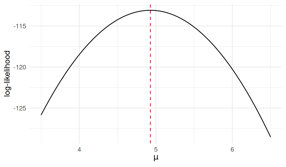
The likelihood is peaked at the sample mean — that is the MLE.

3. Assumptions

Normal model: iid, constant σ. Poisson model: iid counts, constant rate over a fixed exposure. Fisher information is evaluated at the MLE for the Wald standard error.

4. Conduct

Normal mean by MLE

mle_mu <- mean(x)
# Fisher information for mu in normal with known sigma is n / sigma^2.
I_mu <- n / sigma^2
se_mu <- 1 / sqrt(I_mu)
ci_mu <- mle_mu + c(-1, 1) * qnorm(0.975) * se_mu
tibble(mle = mle_mu, se = se_mu,
       ci_low = ci_mu[1], ci_high = ci_mu[2])

# A tibble: 1 × 4
    mle    se ci_low ci_high
  <dbl> <dbl>  <dbl>   <dbl>
1  4.93 0.283   4.37    5.48

Normal mean by numeric optimisation (sanity check)

nll <- function(mu) -sum(dnorm(x, mu, sigma, log = TRUE))
opt <- optim(0, nll, method = "Brent", lower = 0, upper = 10, hessian = TRUE)
opt$par        # MLE

[1] 4.928656

sqrt(1 / opt$hessian[1, 1])  # SE from observed information

[1] 0.2828427

Poisson rate by MLE

y <- rpois(100, lambda = 3.2)
mle_lambda <- mean(y)
# Fisher information for lambda: n / lambda. At MLE use 1/mle_lambda per obs.
I_lambda <- length(y) / mle_lambda
se_lambda <- 1 / sqrt(I_lambda)
ci_lambda <- mle_lambda + c(-1, 1) * qnorm(0.975) * se_lambda
tibble(mle = mle_lambda, se = se_lambda,
       ci_low = ci_lambda[1], ci_high = ci_lambda[2])

# A tibble: 1 × 4
    mle    se ci_low ci_high
  <dbl> <dbl>  <dbl>   <dbl>
1  3.24  0.18   2.89    3.59

Likelihood surface for a two-parameter model (μ, σ)

surf <- expand_grid(
  mu = seq(3.5, 6.5, length.out = 80),
  s  = seq(1, 3.5, length.out = 80)
) |>
  rowwise() |>
  mutate(ll = sum(dnorm(x, mu, s, log = TRUE))) |>
  ungroup()

ggplot(surf, aes(mu, s, fill = ll)) +
  geom_tile() +
  geom_contour(aes(z = ll), colour = "white") +
  scale_fill_viridis_c() +
  labs(x = expression(mu), y = expression(sigma), fill = "log-L")

5. Concluding statement

The MLE of the normal mean from n = 50 observations at σ = 2 was 4.929 (Fisher-information SE = 0.283; 95% Wald CI 4.37 to 5.48), recovering the true μ = 5. The MLE of the Poisson rate from n = 100 observations was 3.24 (SE 0.18; CI 2.89 to 3.59). Observed-information SEs from optim agreed with the expected-information calculation.

The MLE is the general-purpose engine behind linear regression, logistic regression, Cox models, and the bulk of parametric inference in this course. The machinery — likelihood, information, SE — is the same in each case.

Draw the likelihood surface by hand first. The contour plot is the intuition the students should take away.

Common pitfalls

• Reporting a Wald CI when the sample is small. Profile CIs are more accurate in that regime.
• Evaluating Fisher information at a wrong value of the parameter. Use the MLE.
• Forgetting that the MLE is not always unbiased for finite n — only asymptotically.

Further reading

• Casella G, Berger RL. Statistical Inference, chapter on point estimation.
• Cox DR. Principles of Statistical Inference.

Session info

sessionInfo()

R version 4.4.1 (2024-06-14)
Platform: x86_64-pc-linux-gnu
Running under: Ubuntu 24.04.4 LTS

Matrix products: default
BLAS:   /usr/lib/x86_64-linux-gnu/openblas-pthread/libblas.so.3 
LAPACK: /usr/lib/x86_64-linux-gnu/openblas-pthread/libopenblasp-r0.3.26.so;  LAPACK version 3.12.0

locale:
 [1] LC_CTYPE=C.UTF-8       LC_NUMERIC=C           LC_TIME=C.UTF-8       
 [4] LC_COLLATE=C.UTF-8     LC_MONETARY=C.UTF-8    LC_MESSAGES=C.UTF-8   
 [7] LC_PAPER=C.UTF-8       LC_NAME=C              LC_ADDRESS=C          
[10] LC_TELEPHONE=C         LC_MEASUREMENT=C.UTF-8 LC_IDENTIFICATION=C   

time zone: UTC
tzcode source: system (glibc)

attached base packages:
[1] stats     graphics  grDevices utils     datasets  methods   base     

other attached packages:
 [1] lubridate_1.9.5 forcats_1.0.1   stringr_1.6.0   dplyr_1.2.1    
 [5] purrr_1.2.2     readr_2.2.0     tidyr_1.3.2     tibble_3.3.1   
 [9] ggplot2_4.0.3   tidyverse_2.0.0

loaded via a namespace (and not attached):
 [1] gtable_0.3.6       jsonlite_2.0.0     compiler_4.4.1     tidyselect_1.2.1  
 [5] scales_1.4.0       yaml_2.3.12        fastmap_1.2.0      R6_2.6.1          
 [9] labeling_0.4.3     generics_0.1.4     isoband_0.3.0      knitr_1.51        
[13] htmlwidgets_1.6.4  pillar_1.11.1      RColorBrewer_1.1-3 tzdb_0.5.0        
[17] rlang_1.2.0        stringi_1.8.7      xfun_0.57          S7_0.2.2          
[21] otel_0.2.0         viridisLite_0.4.3  timechange_0.4.0   cli_3.6.6         
[25] withr_3.0.2        magrittr_2.0.5     digest_0.6.39      grid_4.4.1        
[29] hms_1.1.4          lifecycle_1.0.5    vctrs_0.7.3        evaluate_1.0.5    
[33] glue_1.8.1         farver_2.1.2       rmarkdown_2.31     tools_4.4.1       
[37] pkgconfig_2.0.3    htmltools_0.5.9