Week 3, Session 4 — One-sample t-test and one-proportion test

Course 1 — #courses

R. Heller

Note

Inference labs use the five-step template: Hypothesis → Visualise → Assumptions → Conduct → Conclude.

Learning objectives

• State a one-sample null and alternative hypothesis for a continuous outcome and for a proportion.
• Run t.test(mu = ) and prop.test() / binom.test() and interpret the output.
• Apply the full five-step inference template in one working pass.

Prerequisites

Labs 2.5, 3.3.

Background

The one-sample t-test asks whether the mean of a continuous outcome differs from a pre-specified value μ₀. It is the inference analogue of Table 1: a single-column calculation asking whether the sample is consistent with a named population mean. The test statistic is (x̄ − μ₀) / (s/√n), compared to a t distribution on n − 1 degrees of freedom.

The one-proportion test does the same for a binary outcome. When the sample is large we use prop.test(), which is a Wald-type test based on the normal approximation to the binomial; when the sample is small, binom.test() gives an exact test based on the binomial PMF. Both return a p-value, a point estimate, and a CI.

These are the simplest tests in the course, but the five-step template — hypothesis, visualise, assumptions, conduct, conclude — is the same template used in every later inference lab. Getting the template into muscle memory here pays dividends throughout the rest of the course.

Setup

library(tidyverse)
set.seed(42)
theme_set(theme_minimal(base_size = 12))

1. Hypothesis

Scenario A (continuous): fasting blood glucose in a random sample of n = 40 patients from a clinic. Reference mean μ₀ = 95 mg/dL in a healthy population. Two-sided test.

• H0: μ = 95
• H1: μ ≠ 95
• α = 0.05

Scenario B (proportion): of 120 patients offered a new screening programme, k = 78 accepted. Reference acceptance rate π₀ = 0.60.

• H0: π = 0.60
• H1: π ≠ 0.60
• α = 0.05

2. Visualise

n <- 40
glucose <- rnorm(n, mean = 100, sd = 12)

tibble(glucose) |>
  ggplot(aes(glucose)) +
  geom_histogram(bins = 15, fill = "grey60", colour = "white") +
  geom_vline(xintercept = 95, linetype = 2) +
  geom_vline(xintercept = mean(glucose), colour = "firebrick") +
  labs(x = "Fasting glucose (mg/dL)", y = "Count")

accept <- 78
total  <- 120
tibble(state = c("accepted", "declined"),
       count = c(accept, total - accept))

# A tibble: 2 × 2
  state    count
  <chr>    <dbl>
1 accepted    78
2 declined    42

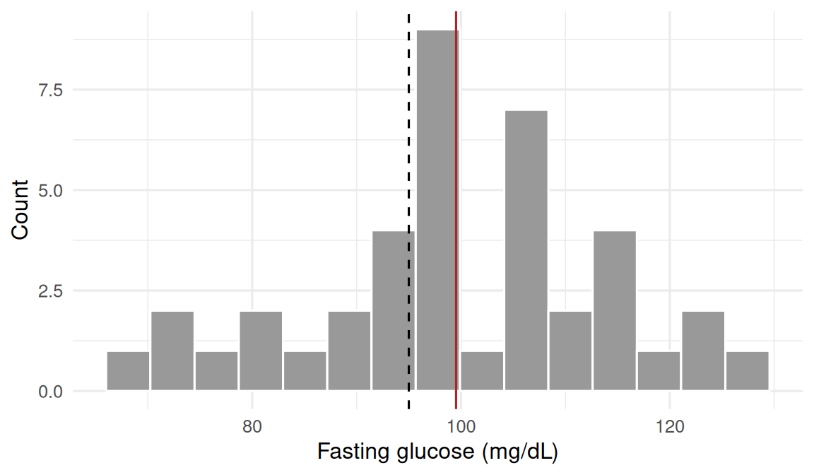
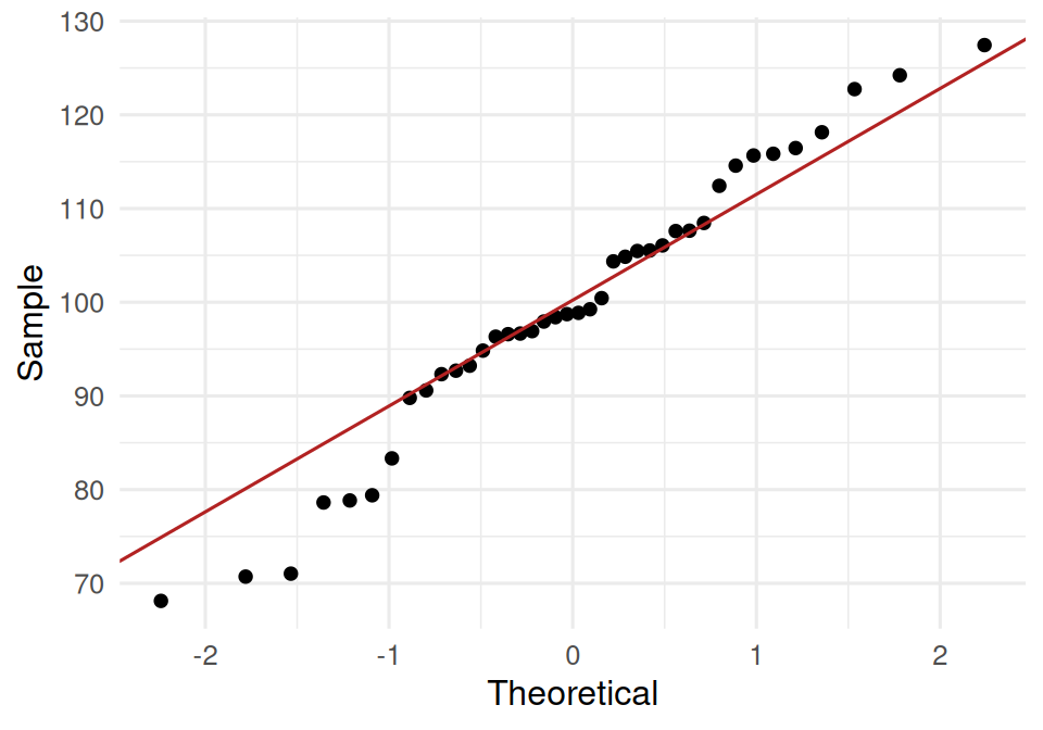
3. Assumptions

t-test: approximate normality of the sample mean, which — by the central limit theorem — holds for n = 40 unless the underlying distribution is strongly skewed. Check with a Q-Q plot.

tibble(glucose) |>
  ggplot(aes(sample = glucose)) +
  stat_qq() + stat_qq_line(colour = "firebrick") +
  labs(x = "Theoretical", y = "Sample")

Proportion test: independent binary trials, same success probability. For prop.test the large-sample normal approximation needs np₀ ≥ 5 and n(1 − p₀) ≥ 5; both are satisfied.

4. Conduct

tt <- t.test(glucose, mu = 95)
tt

    One Sample t-test

data:  glucose
t = 1.9513, df = 39, p-value = 0.05824
alternative hypothesis: true mean is not equal to 95
95 percent confidence interval:
  94.83431 104.21683
sample estimates:
mean of x 
 99.52557 

pt_large <- prop.test(x = accept, n = total, p = 0.60)
pt_exact <- binom.test(x = accept, n = total, p = 0.60)
list(prop_test = pt_large, binom_test = pt_exact)

$prop_test

    1-sample proportions test with continuity correction

data:  accept out of total, null probability 0.6
X-squared = 1.0503, df = 1, p-value = 0.3054
alternative hypothesis: true p is not equal to 0.6
95 percent confidence interval:
 0.5569559 0.7332917
sample estimates:
   p 
0.65 


$binom_test

    Exact binomial test

data:  accept and total
number of successes = 78, number of trials = 120, p-value = 0.3054
alternative hypothesis: true probability of success is not equal to 0.6
95 percent confidence interval:
 0.5576053 0.7347977
sample estimates:
probability of success 
                  0.65 

5. Concluding statement

Scenario A. In a sample of 40 patients, mean fasting glucose was 99.5 mg/dL (SD 14.7). The one-sample t-test against μ₀ = 95 gave t(39) = 1.95, p = 0.058, mean difference 4.5 (95% CI -0.2 to 9.2).

Scenario B. Acceptance was 78 of 120 (65%); the exact one-proportion test against π₀ = 0.60 gave p = 0.31, 95% CI 0.56 to 0.73.

The two scenarios share a template. The glossary changes — mean and SD for continuous, count and proportion for binary — but the five steps are the same.

Make the template rigid here. In subsequent labs the students will riff on it; the rigidity at this stage is the anchor.

Common pitfalls

• Running a one-sided test to “rescue” a borderline two-sided p-value.
• Reporting the p-value without the mean difference and its CI.
• Using prop.test when the expected count of either outcome is very small; use binom.test there.

Further reading

• Rosner B. Fundamentals of Biostatistics, chapter on one-sample inference.
• Altman DG, Confidence intervals rather than p values, BMJ 1986.

Session info

sessionInfo()

R version 4.4.1 (2024-06-14)
Platform: x86_64-pc-linux-gnu
Running under: Ubuntu 24.04.4 LTS

Matrix products: default
BLAS:   /usr/lib/x86_64-linux-gnu/openblas-pthread/libblas.so.3 
LAPACK: /usr/lib/x86_64-linux-gnu/openblas-pthread/libopenblasp-r0.3.26.so;  LAPACK version 3.12.0

locale:
 [1] LC_CTYPE=C.UTF-8       LC_NUMERIC=C           LC_TIME=C.UTF-8       
 [4] LC_COLLATE=C.UTF-8     LC_MONETARY=C.UTF-8    LC_MESSAGES=C.UTF-8   
 [7] LC_PAPER=C.UTF-8       LC_NAME=C              LC_ADDRESS=C          
[10] LC_TELEPHONE=C         LC_MEASUREMENT=C.UTF-8 LC_IDENTIFICATION=C   

time zone: UTC
tzcode source: system (glibc)

attached base packages:
[1] stats     graphics  grDevices utils     datasets  methods   base     

other attached packages:
 [1] lubridate_1.9.5 forcats_1.0.1   stringr_1.6.0   dplyr_1.2.1    
 [5] purrr_1.2.2     readr_2.2.0     tidyr_1.3.2     tibble_3.3.1   
 [9] ggplot2_4.0.3   tidyverse_2.0.0

loaded via a namespace (and not attached):
 [1] gtable_0.3.6       jsonlite_2.0.0     compiler_4.4.1     tidyselect_1.2.1  
 [5] scales_1.4.0       yaml_2.3.12        fastmap_1.2.0      R6_2.6.1          
 [9] labeling_0.4.3     generics_0.1.4     knitr_1.51         htmlwidgets_1.6.4 
[13] pillar_1.11.1      RColorBrewer_1.1-3 tzdb_0.5.0         rlang_1.2.0       
[17] utf8_1.2.6         stringi_1.8.7      xfun_0.57          S7_0.2.2          
[21] otel_0.2.0         timechange_0.4.0   cli_3.6.6          withr_3.0.2       
[25] magrittr_2.0.5     digest_0.6.39      grid_4.4.1         hms_1.1.4         
[29] lifecycle_1.0.5    vctrs_0.7.3        evaluate_1.0.5     glue_1.8.1        
[33] farver_2.1.2       rmarkdown_2.31     tools_4.4.1        pkgconfig_2.0.3   
[37] htmltools_0.5.9