Week 3, Session 5 — Hypothesis testing, p-values, type I/II errors

Course 1 — #courses

R. Heller

Note

Inference labs use the five-step template: Hypothesis → Visualise → Assumptions → Conduct → Conclude.

Learning objectives

• State what a p-value is, and — just as importantly — what it is not.
• Demonstrate by simulation that p-values are uniform under H0.
• Quantify type I error, type II error, and power, and show their relationship.

Prerequisites

Lab 3.4.

Background

A p-value is the probability of observing a test statistic at least as extreme as the one computed, under the null hypothesis. It is not the probability that the null is true. It is not the probability that the result was due to chance. Both of those are common, plausible misreadings; both are wrong. The p-value is a function of the data under one specific hypothetical: if H0 were true, how often would we see this much apparent signal?

Under H0, the p-value is uniformly distributed on [0, 1]. This is a direct consequence of the probability integral transform, and it is the reason the familiar threshold 0.05 gives a 5% type I error rate when applied across many independent tests of true nulls.

Type I error is the rate of false positives; type II error is the rate of false negatives. Power is 1 − type II error: the probability of detecting a true effect. Power depends on the effect size, the variability, the sample size, and α. Increasing n buys you power; increasing α buys you power at the cost of more false positives.

Setup

library(tidyverse)
set.seed(42)
theme_set(theme_minimal(base_size = 12))

1. Hypothesis

The lab has two claims to verify:

1. Under H0 (no effect), the p-value from a two-sample t-test is uniform on [0, 1].
2. Under H1 (effect present), the probability of rejecting H0 depends on sample size and effect size.

2. Visualise

Generate many datasets with no effect, run a t-test on each, and plot the distribution of p-values.

simulate_pvals <- function(n_per_group = 30, delta = 0, B = 5000) {
  replicate(B, {
    a <- rnorm(n_per_group, 0, 1)
    b <- rnorm(n_per_group, delta, 1)
    t.test(a, b)$p.value
  })
}
p_h0 <- simulate_pvals(30, delta = 0)

tibble(p = p_h0) |>
  ggplot(aes(p)) +
  geom_histogram(bins = 20, fill = "grey60", colour = "white") +
  geom_hline(yintercept = length(p_h0) / 20,
             linetype = 2, colour = "firebrick") +
  labs(x = "p-value under H0", y = "Count")

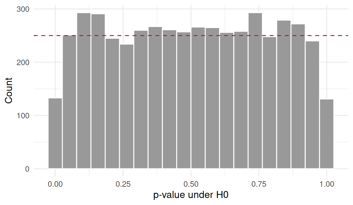
Flat histogram. Any other shape is a sign the test is misspecified.

3. Assumptions

The claim that p-values are uniform under H0 requires that H0 be correctly specified — the distributional assumptions of the test must hold. If the t-test is applied to strongly skewed data at small n, the histogram will not be flat, and the type I error will depart from α.

4. Conduct

Type I error rate

type_I <- mean(p_h0 < 0.05)
type_I

[1] 0.0522

Close to the nominal 0.05.

Power under H1 (effect size 0.5, n per group 30)

p_h1 <- simulate_pvals(30, delta = 0.5)
power_obs <- mean(p_h1 < 0.05)
power_obs

[1] 0.4902

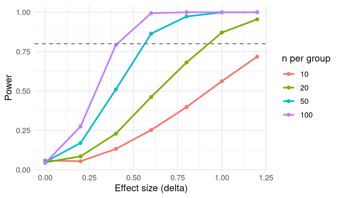
Power by effect size and sample size

grid <- expand_grid(
  n = c(10, 20, 50, 100),
  delta = seq(0, 1.2, by = 0.2)
)
grid$power <- with(grid, mapply(function(nn, dd) {
  mean(simulate_pvals(nn, dd, B = 1000) < 0.05)
}, n, delta))

grid |>
  ggplot(aes(delta, power, colour = factor(n))) +
  geom_line(linewidth = 1) +
  geom_point() +
  geom_hline(yintercept = 0.8, linetype = 2, colour = "grey40") +
  labs(x = "Effect size (delta)", y = "Power",
       colour = "n per group")

5. Concluding statement

In 5000 simulated datasets with no true effect, the empirical type I error rate of the two-sample t-test was 0.052 (nominal 0.05), and the p-value histogram was flat as theory requires. With a true effect δ = 0.5 at n = 30 per group, the empirical power was 0.49. Power grew with both effect size and sample size as expected; 80% power at δ = 0.5 required roughly n = 65 per group.

A p-value is a random variable, uniform under H0. The common bar of 0.05 is a convention, not a discovery about nature, and rejecting results above it is a statement about rates of evidence in a long run of studies — not about the truth of any single study.

The flat histogram is the single most important picture in the course. It is the demonstration that we understand what a p-value means.

Common pitfalls

• Reporting p = 0.051 as “not significant” and p = 0.049 as “significant” as if the dichotomy were informative.
• Confusing P(data | H0) with P(H0 | data).
• Running many tests without adjustment and reporting the smallest p-value.
• Declaring “no effect” when a non-significant p-value comes from an underpowered study.

Further reading

• Wasserstein RL, Lazar NA (2016). The ASA’s Statement on p-Values.
• Greenland S et al. (2016). Statistical tests, P values, confidence intervals, and power: a guide to misinterpretations.

Session info

sessionInfo()

R version 4.4.1 (2024-06-14)
Platform: x86_64-pc-linux-gnu
Running under: Ubuntu 24.04.4 LTS

Matrix products: default
BLAS:   /usr/lib/x86_64-linux-gnu/openblas-pthread/libblas.so.3 
LAPACK: /usr/lib/x86_64-linux-gnu/openblas-pthread/libopenblasp-r0.3.26.so;  LAPACK version 3.12.0

locale:
 [1] LC_CTYPE=C.UTF-8       LC_NUMERIC=C           LC_TIME=C.UTF-8       
 [4] LC_COLLATE=C.UTF-8     LC_MONETARY=C.UTF-8    LC_MESSAGES=C.UTF-8   
 [7] LC_PAPER=C.UTF-8       LC_NAME=C              LC_ADDRESS=C          
[10] LC_TELEPHONE=C         LC_MEASUREMENT=C.UTF-8 LC_IDENTIFICATION=C   

time zone: UTC
tzcode source: system (glibc)

attached base packages:
[1] stats     graphics  grDevices utils     datasets  methods   base     

other attached packages:
 [1] lubridate_1.9.5 forcats_1.0.1   stringr_1.6.0   dplyr_1.2.1    
 [5] purrr_1.2.2     readr_2.2.0     tidyr_1.3.2     tibble_3.3.1   
 [9] ggplot2_4.0.3   tidyverse_2.0.0

loaded via a namespace (and not attached):
 [1] gtable_0.3.6       jsonlite_2.0.0     compiler_4.4.1     tidyselect_1.2.1  
 [5] scales_1.4.0       yaml_2.3.12        fastmap_1.2.0      R6_2.6.1          
 [9] labeling_0.4.3     generics_0.1.4     knitr_1.51         htmlwidgets_1.6.4 
[13] pillar_1.11.1      RColorBrewer_1.1-3 tzdb_0.5.0         rlang_1.2.0       
[17] stringi_1.8.7      xfun_0.57          S7_0.2.2           otel_0.2.0        
[21] timechange_0.4.0   cli_3.6.6          withr_3.0.2        magrittr_2.0.5    
[25] digest_0.6.39      grid_4.4.1         hms_1.1.4          lifecycle_1.0.5   
[29] vctrs_0.7.3        evaluate_1.0.5     glue_1.8.1         farver_2.1.2      
[33] rmarkdown_2.31     tools_4.4.1        pkgconfig_2.0.3    htmltools_0.5.9