Week 4, Session 2 — Two proportions, chi-square, risk and odds

Course 1 — #courses

Author

R. Heller

Note

Inference labs use the five-step template: Hypothesis → Visualise → Assumptions → Conduct → Conclude.

Learning objectives

Compare two proportions with prop.test() and fisher.test() and say when each is preferred.
Compute risk ratio, odds ratio, and risk difference with confidence intervals.
Run a chi-square goodness-of-fit test against a named distribution.

Prerequisites

Labs 2.4, 3.4.

Background

Two-proportion tests ask whether the rate of an event differs between two groups. In a 2x2 table, two exposure groups (say, treatment and control) each produce a fraction of events. The chi-square test compares the observed counts to those expected under independence; Fisher’s exact test computes the probability of a table as extreme or more extreme directly from the hypergeometric distribution and is preferred when expected cell counts are small.

The effect can be expressed in several ways. The risk difference is the difference of the two proportions. The risk ratio is their ratio — the event rate in the treated group, relative to control. The odds ratio is the ratio of the odds. In a case-control study the risk ratio is not directly estimable; the odds ratio is. In a cohort study both are estimable and the risk ratio is usually more intuitive.

Goodness-of-fit tests compare a vector of observed counts to a vector of expected proportions under a named distribution — whether a die is fair, whether a set of genotype frequencies matches Hardy-Weinberg, whether arrivals over an hour are Poisson. The test statistic is the same chi-square; the interpretation is “is the distribution consistent with a named model?”

Setup

library(tidyverse)
set.seed(42)
theme_set(theme_minimal(base_size = 12))

1. Hypothesis

Two-by-two: treatment vs control, outcome event vs none.

H0: event rate is independent of treatment.
H1: rates differ.
α = 0.05.

2. Visualise

Simulate: 200 per arm, event rate 0.25 in control, 0.15 in treatment.

n_per <- 200
sim <- tibble(
  arm = rep(c("control", "treatment"), each = n_per),
  event = c(rbinom(n_per, 1, 0.25),
            rbinom(n_per, 1, 0.15))
)
tab <- table(arm = sim$arm, event = sim$event)
tab

           event
arm           0   1
  control   148  52
  treatment 167  33

as_tibble(tab) |>
  mutate(arm = factor(arm, levels = c("control", "treatment")),
         event = recode(event, `0` = "no event", `1` = "event")) |>
  ggplot(aes(arm, n, fill = event)) +
  geom_col(position = "fill", alpha = 0.7) +
  labs(x = NULL, y = "Proportion", fill = NULL)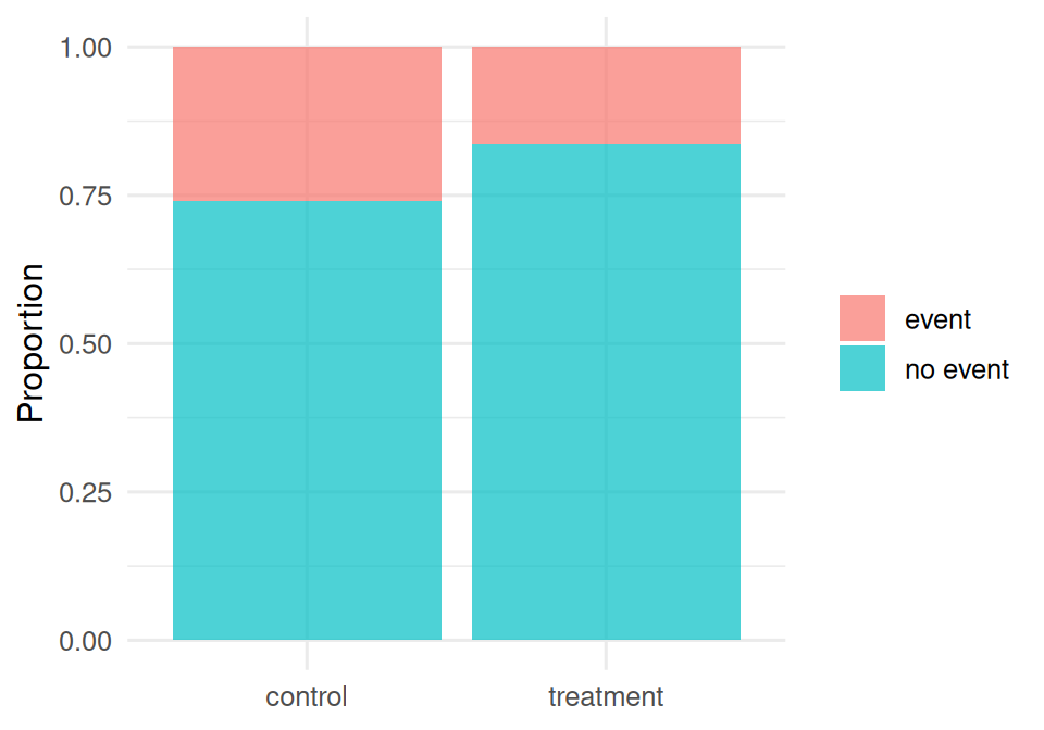

3. Assumptions

Chi-square requires expected cell counts ≥ 5. Fisher has no such constraint and is exact at any size. Random assignment or representative sampling is assumed. Independence of observations is essential.

chisq.test(tab)$expected

           event
arm             0    1
  control   157.5 42.5
  treatment 157.5 42.5

All expected counts large; chi-square is appropriate.

4. Conduct

ct <- chisq.test(tab, correct = FALSE)
ft <- fisher.test(tab)
pt <- prop.test(x = tab[, "1"], n = rowSums(tab), correct = FALSE)
list(chisq = ct, fisher = ft, prop = pt)

$chisq

    Pearson's Chi-squared test

data:  tab
X-squared = 5.3931, df = 1, p-value = 0.02022


$fisher

    Fisher's Exact Test for Count Data

data:  tab
p-value = 0.02743
alternative hypothesis: true odds ratio is not equal to 1
95 percent confidence interval:
 0.3331919 0.9418077
sample estimates:
odds ratio 
 0.5632336 


$prop

    2-sample test for equality of proportions without continuity correction

data:  tab[, "1"] out of rowSums(tab)
X-squared = 5.3931, df = 1, p-value = 0.02022
alternative hypothesis: two.sided
95 percent confidence interval:
 0.01536478 0.17463522
sample estimates:
prop 1 prop 2 
 0.260  0.165

Effect sizes: RD, RR, OR

p_ctrl <- tab["control",   "1"] / sum(tab["control", ])
p_trt  <- tab["treatment", "1"] / sum(tab["treatment", ])

rd <- p_trt - p_ctrl

rr <- p_trt / p_ctrl
# Log-based Wald CI for RR
se_log_rr <- sqrt(
  (1 - p_trt)  / (p_trt  * sum(tab["treatment", ])) +
  (1 - p_ctrl) / (p_ctrl * sum(tab["control",   ]))
)
ci_rr <- exp(log(rr) + c(-1, 1) * qnorm(0.975) * se_log_rr)

or <- (tab["treatment", "1"] * tab["control", "0"]) /
      (tab["treatment", "0"] * tab["control", "1"])
se_log_or <- sqrt(sum(1 / tab))
ci_or <- exp(log(or) + c(-1, 1) * qnorm(0.975) * se_log_or)

tibble(effect = c("RD", "RR", "OR"),
       est = c(rd, rr, or),
       ci_low = c(pt$conf.int[1], ci_rr[1], ci_or[1]),
       ci_high = c(pt$conf.int[2], ci_rr[2], ci_or[2]))

# A tibble: 3 × 4
  effect    est ci_low ci_high
  <chr>   <dbl>  <dbl>   <dbl>
1 RD     -0.095 0.0154   0.175
2 RR      0.635 0.430    0.937
3 OR      0.562 0.345    0.917

Goodness-of-fit example

Test whether 600 simulated genotype counts match Hardy-Weinberg proportions at allele frequency 0.3.

obs <- c(AA = 260, Aa = 290, aa = 50)
pAA <- 0.7^2; paa <- 0.3^2; pAa <- 2 * 0.7 * 0.3
exp_probs <- c(AA = pAA, Aa = pAa, aa = paa)
gof <- chisq.test(obs, p = exp_probs)
gof


    Chi-squared test for given probabilities

data:  obs
X-squared = 9.9584, df = 2, p-value = 0.006879

5. Concluding statement

Event rates were 0.26 in control and 0.165 in treatment (RD -0.095; RR 0.63, 95% CI 0.43 to 0.94; OR 0.56, 95% CI 0.34 to 0.92). Chi-square test χ² = 5.39, df = 1, p = 0.02. The Hardy-Weinberg goodness-of-fit test on simulated genotypes gave χ² = 9.96 (df = 2, p = 0.0069).

Report RR or OR alongside the p-value. In a cohort design prefer RR, which is the quantity clinicians translate directly to practice.

Remind students that OR and RR diverge when the outcome is common. This is the single most-quoted basic epidemiology point in Course 2.

Common pitfalls

Reporting an OR when a RR is meaningful and more interpretable.
Using the continuity correction (the default in prop.test and chisq.test) by habit; it is conservative.
Running a chi-square when expected counts are small; use Fisher.
Treating independent observations as if repeated measures weren’t.

Session info

sessionInfo()

R version 4.4.1 (2024-06-14)
Platform: x86_64-pc-linux-gnu
Running under: Ubuntu 24.04.4 LTS

Matrix products: default
BLAS:   /usr/lib/x86_64-linux-gnu/openblas-pthread/libblas.so.3 
LAPACK: /usr/lib/x86_64-linux-gnu/openblas-pthread/libopenblasp-r0.3.26.so;  LAPACK version 3.12.0

locale:
 [1] LC_CTYPE=C.UTF-8       LC_NUMERIC=C           LC_TIME=C.UTF-8       
 [4] LC_COLLATE=C.UTF-8     LC_MONETARY=C.UTF-8    LC_MESSAGES=C.UTF-8   
 [7] LC_PAPER=C.UTF-8       LC_NAME=C              LC_ADDRESS=C          
[10] LC_TELEPHONE=C         LC_MEASUREMENT=C.UTF-8 LC_IDENTIFICATION=C   

time zone: UTC
tzcode source: system (glibc)

attached base packages:
[1] stats     graphics  grDevices utils     datasets  methods   base     

other attached packages:
 [1] lubridate_1.9.5 forcats_1.0.1   stringr_1.6.0   dplyr_1.2.1    
 [5] purrr_1.2.2     readr_2.2.0     tidyr_1.3.2     tibble_3.3.1   
 [9] ggplot2_4.0.3   tidyverse_2.0.0

loaded via a namespace (and not attached):
 [1] gtable_0.3.6       jsonlite_2.0.0     compiler_4.4.1     tidyselect_1.2.1  
 [5] scales_1.4.0       yaml_2.3.12        fastmap_1.2.0      R6_2.6.1          
 [9] labeling_0.4.3     generics_0.1.4     knitr_1.51         htmlwidgets_1.6.4 
[13] pillar_1.11.1      RColorBrewer_1.1-3 tzdb_0.5.0         rlang_1.2.0       
[17] utf8_1.2.6         stringi_1.8.7      xfun_0.57          S7_0.2.2          
[21] otel_0.2.0         timechange_0.4.0   cli_3.6.6          withr_3.0.2       
[25] magrittr_2.0.5     digest_0.6.39      grid_4.4.1         hms_1.1.4         
[29] lifecycle_1.0.5    vctrs_0.7.3        evaluate_1.0.5     glue_1.8.1        
[33] farver_2.1.2       rmarkdown_2.31     tools_4.4.1        pkgconfig_2.0.3   
[37] htmltools_0.5.9

Learning objectives

Prerequisites

Background

Setup

1. Hypothesis

2. Visualise

3. Assumptions

4. Conduct

Effect sizes: RD, RR, OR

Goodness-of-fit example

5. Concluding statement

Common pitfalls

Further reading

Session info

Related labs