Week 4, Session 4 — Non-parametric tests

Course 1 — #courses

Author

R. Heller

Note

Inference labs use the five-step template: Hypothesis → Visualise → Assumptions → Conduct → Conclude.

Learning objectives

Choose the right rank-based test for a given design — Wilcoxon signed-rank, Mann-Whitney U, Kruskal-Wallis, sign test.
Run each in base R and interpret the output.
State what null hypothesis each test is really addressing (not always “medians are equal”).

Prerequisites

Labs 3.4, 4.1.

Background

Non-parametric tests make weaker distributional assumptions than the parametric tests that dominate the preceding labs. They tend to test exchangeability of distributions rather than equality of means, and they operate on ranks of the data rather than on the raw values. When the data are heavily skewed, ordinal, or small-sample, the non-parametric alternatives are often the defensible default.

The workhorse set: Wilcoxon signed-rank for paired continuous data; Mann-Whitney U (the wilcox.test with paired = FALSE) for two independent groups; Kruskal-Wallis for three or more groups; sign test as a cruder paired-data option based on the signs of differences alone.

A common mistake is to read these tests as “comparing medians”. They compare distributions. Under additional assumptions — notably that the two groups’ distributions differ only by a location shift — the Mann-Whitney U test does estimate a location shift, but that is a stronger assumption than the test itself requires.

Setup

library(tidyverse)
set.seed(42)
theme_set(theme_minimal(base_size = 12))

1. Hypothesis

Three scenarios:

A. Paired: pre/post in 25 patients, skewed outcome. H0: no shift. B. Independent two-sample: outcome in two arms, skewed. H0: same distribution. C. Three-group comparison: outcome across three centres. H0: same distribution across all three.

2. Visualise

# Scenario A: paired, lognormal-ish
n_a <- 25
pre <- exp(rnorm(n_a, 3, 0.3))
post <- pre * exp(rnorm(n_a, -0.2, 0.3))
df_a <- tibble(id = seq_len(n_a), pre, post,
               delta = post - pre)

# Scenario B: independent two groups, lognormal
n_b <- 30
grp <- rep(c("A", "B"), each = n_b)
y_b <- c(exp(rnorm(n_b, 3, 0.5)),
         exp(rnorm(n_b, 3.4, 0.5)))
df_b <- tibble(grp, y = y_b)

# Scenario C: three groups
n_c <- 25
centre <- rep(c("X", "Y", "Z"), each = n_c)
y_c <- c(exp(rnorm(n_c, 3.0, 0.4)),
         exp(rnorm(n_c, 3.2, 0.4)),
         exp(rnorm(n_c, 3.5, 0.4)))
df_c <- tibble(centre, y = y_c)

df_b |>
  ggplot(aes(grp, y, fill = grp)) +
  geom_boxplot(alpha = 0.6, colour = "grey30") +
  labs(x = NULL, y = "Outcome") +
  theme(legend.position = "none")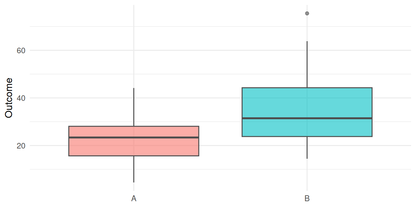

3. Assumptions

Wilcoxon signed-rank: paired observations; differences symmetric around the null. Mann-Whitney U: independent observations within and between groups; if you want a location-shift interpretation, the two distributions should have the same shape. Kruskal-Wallis: independent observations; same-shape assumption extends to all k groups.

4. Conduct

# A: Wilcoxon signed-rank
wt_a <- wilcox.test(df_a$post, df_a$pre, paired = TRUE,
                    conf.int = TRUE)
# Sign test: a simple binomial test on positive differences
signs <- sum(df_a$delta > 0)
sign_test <- binom.test(signs, n_a, p = 0.5)

# B: Mann-Whitney U
wt_b <- wilcox.test(y ~ grp, data = df_b, conf.int = TRUE)

# C: Kruskal-Wallis
kw_c <- kruskal.test(y ~ centre, data = df_c)

list(wilcox_paired = wt_a,
     sign_test = sign_test,
     mann_whitney = wt_b,
     kruskal_wallis = kw_c)

$wilcox_paired

    Wilcoxon signed rank exact test

data:  df_a$post and df_a$pre
V = 29, p-value = 0.000103
alternative hypothesis: true location shift is not equal to 0
95 percent confidence interval:
 -7.462659 -2.298395
sample estimates:
(pseudo)median 
     -4.709926 


$sign_test

    Exact binomial test

data:  signs and n_a
number of successes = 4, number of trials = 25, p-value = 0.0009105
alternative hypothesis: true probability of success is not equal to 0.5
95 percent confidence interval:
 0.04537945 0.36082845
sample estimates:
probability of success 
                  0.16 


$mann_whitney

    Wilcoxon rank sum exact test

data:  y by grp
W = 239, p-value = 0.001525
alternative hypothesis: true location shift is not equal to 0
95 percent confidence interval:
 -17.224482  -3.592832
sample estimates:
difference in location 
              -9.54957 


$kruskal_wallis

    Kruskal-Wallis rank sum test

data:  y by centre
Kruskal-Wallis chi-squared = 27.751, df = 2, p-value = 9.417e-07

Follow-up pairwise comparisons with Holm correction for C:

pairwise.wilcox.test(df_c$y, df_c$centre, p.adjust.method = "holm")


    Pairwise comparisons using Wilcoxon rank sum exact test 

data:  df_c$y and df_c$centre 

  X       Y      
Y 0.01436 -      
Z 1.4e-06 0.00018

P value adjustment method: holm

5. Concluding statement

Paired comparison (A). 25 patients, median change = -4.1; Wilcoxon signed-rank p = 10^{-4}, 95% CI on the Hodges-Lehmann estimate -7.46 to -2.3. Sign test p = 9.1^{-4}.

Two-group (B). Mann-Whitney p = 0.0015, 95% CI -17.22 to -3.59.

Three-group (C). Kruskal-Wallis χ² = 27.75, df = 2, p = 9.4^{-7}. Pairwise Wilcoxon tests with Holm correction indicated the signal lay in the X vs Z contrast.

Non-parametric tests are not free lunches. They trade a modest amount of power (about 5% vs a t-test when the t-test’s assumptions hold) for robustness to distributional misspecification.

Remind the audience that a t-test with log-transformed data is often a cleaner answer than a Wilcoxon on the raw data.

Common pitfalls

Reading a Wilcoxon as a test of medians. It is a test of distributional shift.
Using a rank test when the data are fine on the raw scale, and sacrificing power unnecessarily.
Forgetting to adjust for multiplicity after a Kruskal-Wallis.

Session info

sessionInfo()

R version 4.4.1 (2024-06-14)
Platform: x86_64-pc-linux-gnu
Running under: Ubuntu 24.04.4 LTS

Matrix products: default
BLAS:   /usr/lib/x86_64-linux-gnu/openblas-pthread/libblas.so.3 
LAPACK: /usr/lib/x86_64-linux-gnu/openblas-pthread/libopenblasp-r0.3.26.so;  LAPACK version 3.12.0

locale:
 [1] LC_CTYPE=C.UTF-8       LC_NUMERIC=C           LC_TIME=C.UTF-8       
 [4] LC_COLLATE=C.UTF-8     LC_MONETARY=C.UTF-8    LC_MESSAGES=C.UTF-8   
 [7] LC_PAPER=C.UTF-8       LC_NAME=C              LC_ADDRESS=C          
[10] LC_TELEPHONE=C         LC_MEASUREMENT=C.UTF-8 LC_IDENTIFICATION=C   

time zone: UTC
tzcode source: system (glibc)

attached base packages:
[1] stats     graphics  grDevices utils     datasets  methods   base     

other attached packages:
 [1] lubridate_1.9.5 forcats_1.0.1   stringr_1.6.0   dplyr_1.2.1    
 [5] purrr_1.2.2     readr_2.2.0     tidyr_1.3.2     tibble_3.3.1   
 [9] ggplot2_4.0.3   tidyverse_2.0.0

loaded via a namespace (and not attached):
 [1] gtable_0.3.6       jsonlite_2.0.0     compiler_4.4.1     tidyselect_1.2.1  
 [5] scales_1.4.0       yaml_2.3.12        fastmap_1.2.0      R6_2.6.1          
 [9] labeling_0.4.3     generics_0.1.4     knitr_1.51         htmlwidgets_1.6.4 
[13] pillar_1.11.1      RColorBrewer_1.1-3 tzdb_0.5.0         rlang_1.2.0       
[17] stringi_1.8.7      xfun_0.57          S7_0.2.2           otel_0.2.0        
[21] timechange_0.4.0   cli_3.6.6          withr_3.0.2        magrittr_2.0.5    
[25] digest_0.6.39      grid_4.4.1         hms_1.1.4          lifecycle_1.0.5   
[29] vctrs_0.7.3        evaluate_1.0.5     glue_1.8.1         farver_2.1.2      
[33] rmarkdown_2.31     tools_4.4.1        pkgconfig_2.0.3    htmltools_0.5.9

Learning objectives

Prerequisites

Background

Setup

1. Hypothesis

2. Visualise

3. Assumptions

4. Conduct

5. Concluding statement

Common pitfalls

Further reading

Session info

Related labs