Week 4, Session 5 — Sample size, power, and Quarto reporting

Course 1 — #courses

R. Heller

Note

Workflow lab: Goal → Approach → Execution → Check → Report.

Learning objectives

Compute analytic sample size for the core designs covered in Course 1.
Produce the same answer by simulation and understand when each approach is preferable.
Assemble a short Quarto report whose numbers, tables, and figures all regenerate from a single render.

Prerequisites

Courses 1 Weeks 1–4 up to this lab; pwr, gtsummary, and broom installed.

Background

Sample size is one of the few places where applied statistics is consulted before the data exist. A study that is too small cannot distinguish a real effect from noise; a study that is too large wastes participants and money. The four ingredients of a sample-size calculation — effect size, variability, the significance level, and power — translate directly between a clinical protocol and a funding application, and no competent ethics committee will approve a protocol without them.

There are two complementary approaches. Closed-form formulae, packaged in pwr and friends, are fast, transparent, and correct for the textbook designs: one- and two-sample t-tests, one- and two-proportion tests, correlation, and ANOVA. Simulation-based power, by contrast, is the honest answer for anything the textbooks skip — mixed models, skewed outcomes, interim analyses — and costs only a few minutes of compute. The habit to build is to compute analytically first, then verify by simulation; if the two disagree, either the formula does not apply to your design or your simulation is wrong, and you need to know which.

Reporting is the other half of this lab. Every number in a well-written report should trace back to the code that produced it. Quarto, with gtsummary for tables and broom::tidy() for model output, makes this nearly automatic.

Setup

library(tidyverse)
library(pwr)
library(gtsummary)
library(broom)
set.seed(42)
theme_set(theme_minimal(base_size = 12))

1. Goal

Plan a hypothetical two-arm trial comparing a new antihypertensive with placebo, choose a sample size with 80% power to detect a 5 mmHg difference at α = 0.05, verify by simulation, and produce a reporting table we can paste into the protocol.

2. Approach

Closed-form first. Cohen’s d for a 5 mmHg effect on a scale with SD 10 mmHg is d = 0.5 — a medium effect by convention.

pwr_calc <- pwr.t.test(
  d = 0.5, power = 0.80, sig.level = 0.05,
  type = "two.sample", alternative = "two.sided"
)
pwr_calc


     Two-sample t test power calculation 

              n = 63.76561
              d = 0.5
      sig.level = 0.05
          power = 0.8
    alternative = two.sided

NOTE: n is number in *each* group

The formula calls for about 64 per arm.

ns <- seq(10, 200, by = 5)
powers <- sapply(ns, function(n) {
  pwr.t.test(n = n, d = 0.5, sig.level = 0.05,
             type = "two.sample")$power
})
tibble(n_per_arm = ns, power = powers) |>
  ggplot(aes(n_per_arm, power)) +
  geom_line(linewidth = 0.8) +
  geom_hline(yintercept = 0.8, linetype = 2, colour = "grey50") +
  labs(x = "N per arm", y = "Power",
       title = "Power curve for d = 0.5, α = 0.05")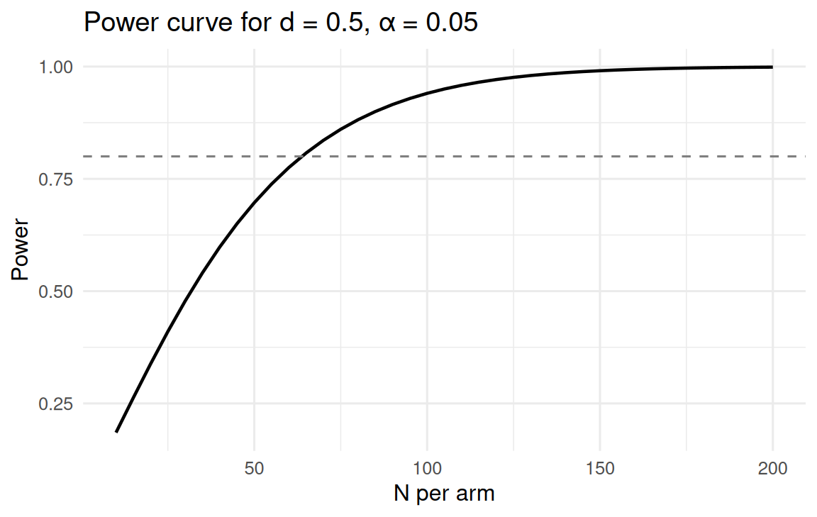

3. Execution

Verify by simulation. A function that runs the trial once and returns the p-value:

sim_trial <- function(n_per_arm, delta = 5, sd = 10) {
  placebo <- rnorm(n_per_arm, 0, sd)
  drug    <- rnorm(n_per_arm, -delta, sd)
  t.test(drug, placebo, var.equal = FALSE)$p.value
}

sim_power <- function(n_per_arm, reps = 500, ...) {
  mean(replicate(reps, sim_trial(n_per_arm, ...)) < 0.05)
}

n_try  <- ceiling(pwr_calc$n)
sim_power(n_try, reps = 1000)

[1] 0.046

Within Monte-Carlo error of the analytic 0.80, as expected.

4. Check

Now imagine the data have been collected. We simulate one realisation and fit the planned analysis.

n <- ceiling(pwr_calc$n)
trial <- tibble(
  arm = rep(c("placebo", "drug"), each = n),
  sbp_change = c(rnorm(n, 0, 10), rnorm(n, -5, 10))
)

fit <- t.test(sbp_change ~ arm, data = trial, var.equal = FALSE)
broom::tidy(fit)

# A tibble: 1 × 10
  estimate estimate1 estimate2 statistic p.value parameter conf.low conf.high
     <dbl>     <dbl>     <dbl>     <dbl>   <dbl>     <dbl>    <dbl>     <dbl>
1   -0.755     -3.58     -2.83    -0.473   0.637      126.    -3.91      2.40
# ℹ 2 more variables: method <chr>, alternative <chr>

5. Report

trial |>
  tbl_summary(
    by = arm,
    statistic = list(all_continuous() ~ "{mean} ({sd})"),
    digits    = all_continuous() ~ 1,
    label     = list(sbp_change = "Change in SBP (mmHg)")
  ) |>
  add_p() |>
  modify_caption("**Table 1. Change in systolic blood pressure, by arm.**")

**Table 1. Change in systolic blood pressure, by arm.**
Characteristic	drug N = 64¹	placebo N = 64¹	p-value²
Change in SBP (mmHg)	-3.6 (8.9)	-2.8 (9.1)	0.7
¹ Mean (SD)
² Wilcoxon rank sum test

In a simulated two-arm trial (n = 64 per arm), mean change in systolic blood pressure was lower in the drug arm than in placebo by -0.8 mmHg (95% CI: -2.4 to 3.9; p = 0.64).

Common pitfalls

Plugging a standardised effect size into a sample-size calculator without stopping to think whether it is plausible in your field.
Quoting “power = 0.8” as a universal target when your decision would justify 0.9 or 0.95.
Reporting a p-value without the effect size and interval that make it interpretable.
Pasting numbers into the manuscript by hand — anything that breaks the render trail will eventually break the numbers.

Session info

sessionInfo()

R version 4.4.1 (2024-06-14)
Platform: x86_64-pc-linux-gnu
Running under: Ubuntu 24.04.4 LTS

Matrix products: default
BLAS:   /usr/lib/x86_64-linux-gnu/openblas-pthread/libblas.so.3 
LAPACK: /usr/lib/x86_64-linux-gnu/openblas-pthread/libopenblasp-r0.3.26.so;  LAPACK version 3.12.0

locale:
 [1] LC_CTYPE=C.UTF-8       LC_NUMERIC=C           LC_TIME=C.UTF-8       
 [4] LC_COLLATE=C.UTF-8     LC_MONETARY=C.UTF-8    LC_MESSAGES=C.UTF-8   
 [7] LC_PAPER=C.UTF-8       LC_NAME=C              LC_ADDRESS=C          
[10] LC_TELEPHONE=C         LC_MEASUREMENT=C.UTF-8 LC_IDENTIFICATION=C   

time zone: UTC
tzcode source: system (glibc)

attached base packages:
[1] stats     graphics  grDevices utils     datasets  methods   base     

other attached packages:
 [1] broom_1.0.12    gtsummary_2.5.0 pwr_1.3-0       lubridate_1.9.5
 [5] forcats_1.0.1   stringr_1.6.0   dplyr_1.2.1     purrr_1.2.2    
 [9] readr_2.2.0     tidyr_1.3.2     tibble_3.3.1    ggplot2_4.0.3  
[13] tidyverse_2.0.0

loaded via a namespace (and not attached):
 [1] gt_1.3.0           sass_0.4.10        utf8_1.2.6         generics_0.1.4    
 [5] xml2_1.5.2         stringi_1.8.7      hms_1.1.4          digest_0.6.39     
 [9] magrittr_2.0.5     evaluate_1.0.5     grid_4.4.1         timechange_0.4.0  
[13] RColorBrewer_1.1-3 cards_0.7.1        fastmap_1.2.0      jsonlite_2.0.0    
[17] cardx_0.3.2        backports_1.5.1    scales_1.4.0       cli_3.6.6         
[21] rlang_1.2.0        litedown_0.9       commonmark_2.0.0   base64enc_0.1-6   
[25] withr_3.0.2        yaml_2.3.12        otel_0.2.0         tools_4.4.1       
[29] tzdb_0.5.0         vctrs_0.7.3        R6_2.6.1           lifecycle_1.0.5   
[33] fs_2.1.0           htmlwidgets_1.6.4  pkgconfig_2.0.3    pillar_1.11.1     
[37] gtable_0.3.6       glue_1.8.1         xfun_0.57          tidyselect_1.2.1  
[41] knitr_1.51         farver_2.1.2       htmltools_0.5.9    rmarkdown_2.31    
[45] labeling_0.4.3     compiler_4.4.1     S7_0.2.2           markdown_2.0

Week 4, Session 5 — Sample size, power, and Quarto reporting

Learning objectives

Prerequisites

Background

Setup

1. Goal

2. Approach

3. Execution

4. Check

5. Report

Common pitfalls

Further reading

Session info