Week 1, Session 2 — Simple linear regression

Course 2 — #courses

R. Heller

Note

Inference labs use the five-step template: Hypothesis → Visualise → Assumptions → Conduct → Conclude.

Learning objectives

• Fit a simple linear regression with lm() and read the output.
• Produce a tidy coefficient table with intervals using broom.
• Draw the fitted line on the scatterplot and express the slope in the units of the variables.

Prerequisites

Session 1 of this week; basic comfort with ggplot2.

Background

Simple linear regression models the mean of a response Y as a linear function of a single predictor X. The model is Y = β₀ + β₁X + ε with the error term ε assumed independent, zero-mean, and of constant variance. The slope β₁ is the expected change in Y for a one-unit change in X; the intercept β₀ is the expected Y at X = 0, which is sometimes meaningful and sometimes only a device for anchoring the line.

Although the formulas are old, the habits they require are modern: always plot first, always report an interval, and always read the slope back in the units of the variables. A regression coefficient is only useful if the reader can imagine the units on the axis.

The default summary() printout from lm() is dense. A clean way to read a fit is to use broom::tidy() for coefficients and broom::glance() for global quantities such as R² and residual standard error, and then plot the line on the data to sanity-check.

Setup

library(tidyverse)
library(broom)
library(palmerpenguins)
set.seed(42)
theme_set(theme_minimal(base_size = 12))

1. Hypothesis

Among Adelie penguins, does bill length predict body mass?

Null: slope of body mass on bill length is zero. Alternative: slope is non-zero.

2. Visualise

ad <- penguins |>
  filter(species == "Adelie") |>
  drop_na(bill_length_mm, body_mass_g)

ggplot(ad, aes(bill_length_mm, body_mass_g)) +
  geom_point(alpha = 0.6, colour = "grey30") +
  geom_smooth(method = "lm", se = TRUE, colour = "steelblue") +
  labs(x = "Bill length (mm)", y = "Body mass (g)")

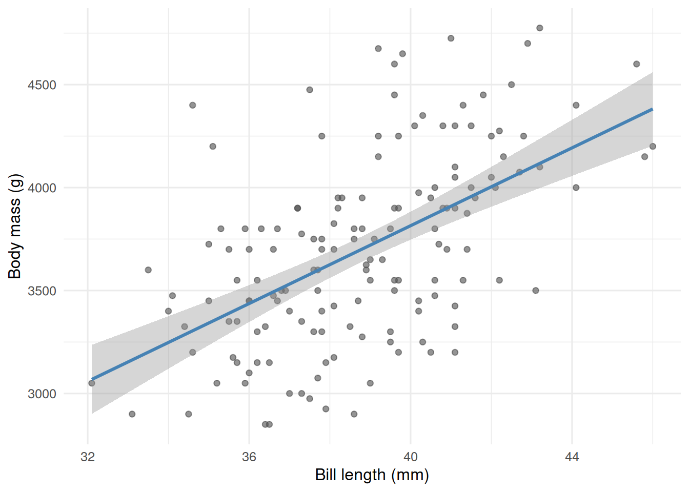
The cloud climbs gently from left to right. The smoothed line is an honest guess at the conditional mean.

3. Assumptions

Linearity, independence, homoscedasticity, and approximate normality of residuals.

fit <- lm(body_mass_g ~ bill_length_mm, data = ad)
par(mfrow = c(2, 2))
plot(fit)

par(mfrow = c(1, 1))

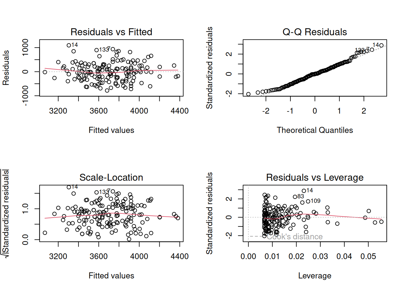
Residuals vs fitted is patternless; QQ is close to straight. No single point dominates.

4. Conduct

tidy(fit, conf.int = TRUE)

# A tibble: 2 × 7
  term           estimate std.error statistic  p.value conf.low conf.high
  <chr>             <dbl>     <dbl>     <dbl>    <dbl>    <dbl>     <dbl>
1 (Intercept)        34.9     458.     0.0761 9.39e- 1   -871.       941.
2 bill_length_mm     94.5      11.8    8.01   2.95e-13     71.2      118.

glance(fit) |> select(r.squared, adj.r.squared, sigma, p.value)

# A tibble: 1 × 4
  r.squared adj.r.squared sigma  p.value
      <dbl>         <dbl> <dbl>    <dbl>
1     0.301         0.297  385. 2.95e-13

slope <- coef(fit)[2]
ci <- confint(fit)[2, ]

5. Concluding statement

Among Adelie penguins (n = 151), each additional mm of bill length was associated with an increase of 94 g in body mass (95% CI: 71 to 118 g; p = 3^{-13}). Bill length explained 30.1% of the variance in body mass.

Point out that R² below 30% is common and fine; the estimate is the story, not the variance explained.

Common pitfalls

• Extrapolating beyond the range of X.
• Interpreting the intercept when X = 0 is nonsensical.
• Quoting R² without reporting the slope and its interval.

Further reading

• Faraway JJ. Linear Models with R, ch. 2.
• Kutner MH et al. Applied Linear Statistical Models, ch. 1–3.
• Weisberg S. Applied Linear Regression.

Session info

sessionInfo()

R version 4.4.1 (2024-06-14)
Platform: x86_64-pc-linux-gnu
Running under: Ubuntu 24.04.4 LTS

Matrix products: default
BLAS:   /usr/lib/x86_64-linux-gnu/openblas-pthread/libblas.so.3 
LAPACK: /usr/lib/x86_64-linux-gnu/openblas-pthread/libopenblasp-r0.3.26.so;  LAPACK version 3.12.0

locale:
 [1] LC_CTYPE=C.UTF-8       LC_NUMERIC=C           LC_TIME=C.UTF-8       
 [4] LC_COLLATE=C.UTF-8     LC_MONETARY=C.UTF-8    LC_MESSAGES=C.UTF-8   
 [7] LC_PAPER=C.UTF-8       LC_NAME=C              LC_ADDRESS=C          
[10] LC_TELEPHONE=C         LC_MEASUREMENT=C.UTF-8 LC_IDENTIFICATION=C   

time zone: UTC
tzcode source: system (glibc)

attached base packages:
[1] stats     graphics  grDevices utils     datasets  methods   base     

other attached packages:
 [1] palmerpenguins_0.1.1 broom_1.0.12         lubridate_1.9.5     
 [4] forcats_1.0.1        stringr_1.6.0        dplyr_1.2.1         
 [7] purrr_1.2.2          readr_2.2.0          tidyr_1.3.2         
[10] tibble_3.3.1         ggplot2_4.0.3        tidyverse_2.0.0     

loaded via a namespace (and not attached):
 [1] Matrix_1.7-0       gtable_0.3.6       jsonlite_2.0.0     compiler_4.4.1    
 [5] tidyselect_1.2.1   splines_4.4.1      scales_1.4.0       yaml_2.3.12       
 [9] fastmap_1.2.0      lattice_0.22-6     R6_2.6.1           labeling_0.4.3    
[13] generics_0.1.4     knitr_1.51         backports_1.5.1    htmlwidgets_1.6.4 
[17] pillar_1.11.1      RColorBrewer_1.1-3 tzdb_0.5.0         rlang_1.2.0       
[21] utf8_1.2.6         stringi_1.8.7      xfun_0.57          S7_0.2.2          
[25] otel_0.2.0         timechange_0.4.0   cli_3.6.6          mgcv_1.9-1        
[29] withr_3.0.2        magrittr_2.0.5     digest_0.6.39      grid_4.4.1        
[33] hms_1.1.4          nlme_3.1-164       lifecycle_1.0.5    vctrs_0.7.3       
[37] evaluate_1.0.5     glue_1.8.1         farver_2.1.2       rmarkdown_2.31    
[41] tools_4.4.1        pkgconfig_2.0.3    htmltools_0.5.9