Week 1, Session 4 — Diagnostics: residuals, QQ, leverage, Cook’s distance, VIF

Course 2 — #courses

R. Heller

Note

Inference labs use the five-step template: Hypothesis → Visualise → Assumptions → Conduct → Conclude.

Learning objectives

• Read the four default plot(lm) diagnostics and say what each is for.
• Identify leverage and influence separately and combine them using Cook’s distance.
• Detect collinearity with VIF and decide when to act on it.

Prerequisites

Sessions 2 and 3 of this week.

Background

Diagnostics are the step in a regression workflow that protects the report from the dataset. A coefficient is only as trustworthy as the assumptions behind it. The four classical plots — residuals vs fitted, QQ, scale-location, and residuals vs leverage — answer four questions: is the mean right, are the errors roughly normal, is the variance constant, and is any single point running the show?

Leverage measures how unusual a point’s predictor values are; influence measures how much the fit changes when that point is removed. Cook’s distance combines the two. A point can have high leverage without high influence if it sits on the regression line, and it can have high influence without spectacular residuals if its predictors are extreme.

The performance::check_model() function wraps many of these ideas in a single call and is increasingly the way teams read diagnostics on screen. car::vif() gives the variance inflation factors; a rule of thumb is that values above 5 deserve attention and above 10 demand it, but rules of thumb are no substitute for thinking about which predictors are truly redundant.

Setup

library(tidyverse)
library(broom)
library(car)
library(performance)
set.seed(42)
theme_set(theme_minimal(base_size = 12))

1. Hypothesis

Simulate a regression with mild heteroscedasticity, a high-leverage point, and two correlated predictors. Ask which diagnostics flag which problem.

2. Visualise

n <- 150
x1 <- rnorm(n, 0, 1)
x2 <- x1 + rnorm(n, 0, 0.3)      # x1 and x2 correlated
x3 <- rnorm(n, 0, 1)
y  <- 1 + 2 * x1 - 1.5 * x2 + 0.5 * x3 + rnorm(n, 0, 1 + 0.4 * abs(x1))
# add one influential point
x1[1] <- 5; x2[1] <- 5; y[1] <- 0
dat <- tibble(y, x1, x2, x3)

ggplot(dat, aes(x1, y)) +
  geom_point(alpha = 0.6) +
  labs(x = "x1", y = "y")

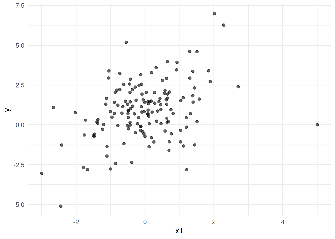
3. Assumptions

fit <- lm(y ~ x1 + x2 + x3, data = dat)
par(mfrow = c(2, 2))
plot(fit)

par(mfrow = c(1, 1))

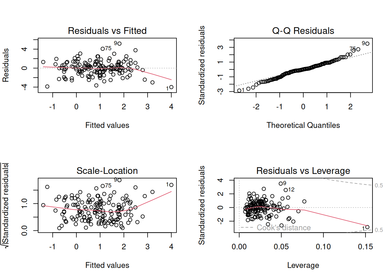
The residuals-vs-fitted plot should show no trend. The QQ plot should track the line. Scale-location should be flat. Residuals-vs-leverage should have no points outside the Cook’s-distance contours.

4. Conduct

Influence diagnostics:

infl <- augment(fit) |> mutate(row = row_number())
infl |> arrange(desc(.cooksd)) |> head(5) |>
  select(row, .fitted, .resid, .hat, .cooksd)

# A tibble: 5 × 5
    row .fitted .resid   .hat .cooksd
  <int>   <dbl>  <dbl>  <dbl>   <dbl>
1     1    4.00  -4.00 0.152   0.369 
2     9    1.81   5.17 0.0493  0.159 
3    12    2.49   3.77 0.0552  0.0958
4    19   -1.23  -3.88 0.0502  0.0909
5    81    3.21  -3.01 0.0643  0.0724

VIF:

vif(fit)

       x1        x2        x3 
15.552171 15.504340  1.014919 

Performance summary:

check_model(fit, check = c("vif", "qq", "outliers", "linearity"))

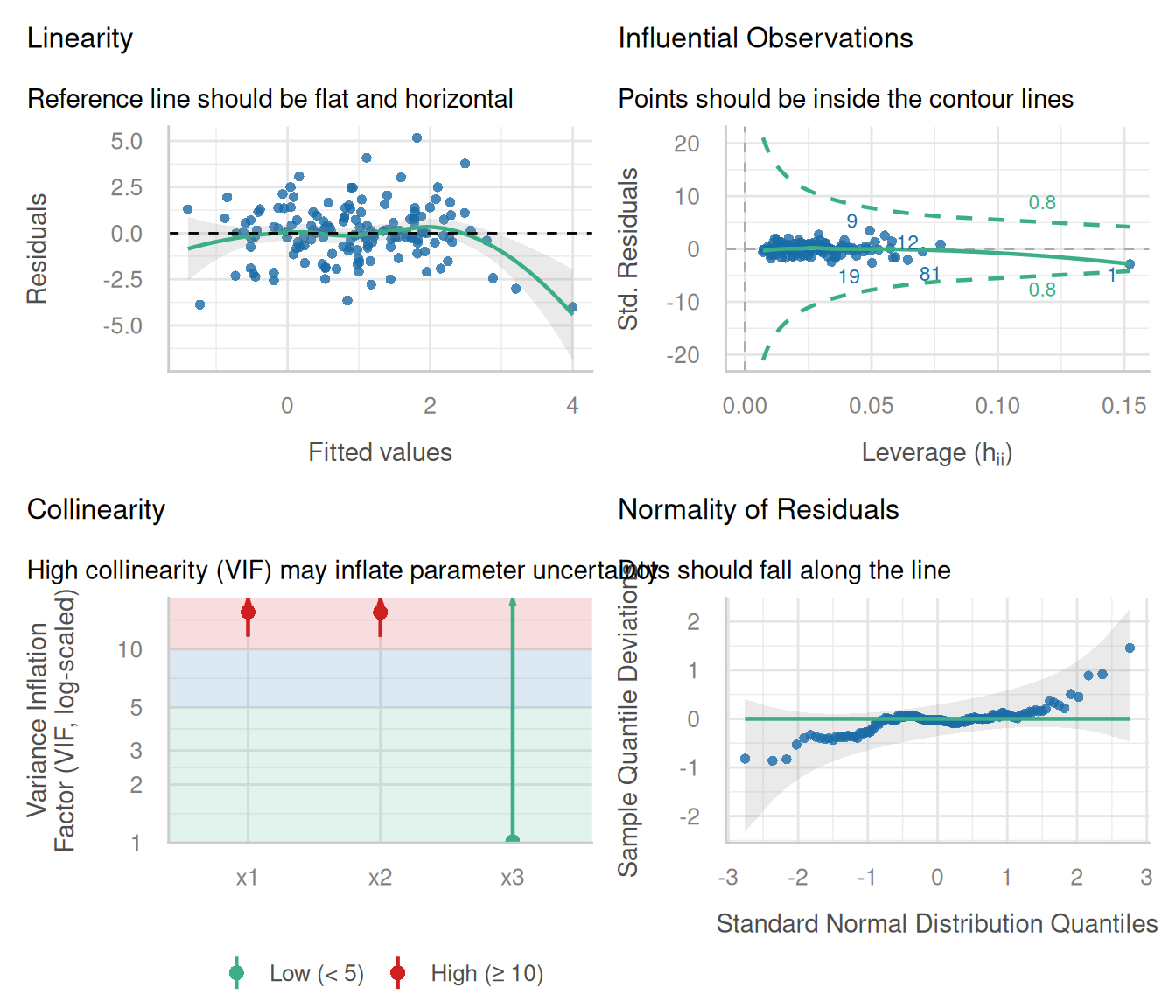
VIF for x1 and x2 should be high; x3 should be fine. The first row (the injected leverage point) should dominate Cook’s distance.

5. Concluding statement

Regression diagnostics identified one high-influence observation (Cook’s D = 0.37) and collinearity between x1 and x2 (VIF = 15.6). Refitting without the influential point or after combining the collinear predictors would be the next step before reporting coefficients.

Stress that diagnostics should be documented, not just inspected: the paper should say which diagnostics were run and what was done about any findings.

Common pitfalls

• Treating a single Cook’s distance number as a verdict. Always look at the plot.
• Solving a VIF problem by dropping one variable at a time when the underlying issue is that two predictors measure the same thing.
• Declaring the assumptions met because the numbers pass. Plot first.

Further reading

• Fox J, Weisberg S. An R Companion to Applied Regression, ch. 8.
• Belsley DA, Kuh E, Welsch RE. Regression Diagnostics.
• Lüdecke D et al. (2021), performance: An R Package for Assessment…

Session info

sessionInfo()

R version 4.4.1 (2024-06-14)
Platform: x86_64-pc-linux-gnu
Running under: Ubuntu 24.04.4 LTS

Matrix products: default
BLAS:   /usr/lib/x86_64-linux-gnu/openblas-pthread/libblas.so.3 
LAPACK: /usr/lib/x86_64-linux-gnu/openblas-pthread/libopenblasp-r0.3.26.so;  LAPACK version 3.12.0

locale:
 [1] LC_CTYPE=C.UTF-8       LC_NUMERIC=C           LC_TIME=C.UTF-8       
 [4] LC_COLLATE=C.UTF-8     LC_MONETARY=C.UTF-8    LC_MESSAGES=C.UTF-8   
 [7] LC_PAPER=C.UTF-8       LC_NAME=C              LC_ADDRESS=C          
[10] LC_TELEPHONE=C         LC_MEASUREMENT=C.UTF-8 LC_IDENTIFICATION=C   

time zone: UTC
tzcode source: system (glibc)

attached base packages:
[1] stats     graphics  grDevices utils     datasets  methods   base     

other attached packages:
 [1] performance_0.16.0 car_3.1-5          carData_3.0-6      broom_1.0.12      
 [5] lubridate_1.9.5    forcats_1.0.1      stringr_1.6.0      dplyr_1.2.1       
 [9] purrr_1.2.2        readr_2.2.0        tidyr_1.3.2        tibble_3.3.1      
[13] ggplot2_4.0.3      tidyverse_2.0.0   

loaded via a namespace (and not attached):
 [1] gtable_0.3.6            xfun_0.57               bayestestR_0.17.0      
 [4] twosamples_2.0.1        caTools_1.18.3          htmlwidgets_1.6.4      
 [7] insight_1.5.0           ggrepel_0.9.8           lattice_0.22-6         
[10] tzdb_0.5.0              bitops_1.0-9            vctrs_0.7.3            
[13] tools_4.4.1             generics_0.1.4          datawizard_1.3.1       
[16] parallel_4.4.1          pbmcapply_1.5.1         DEoptimR_1.1-4         
[19] pkgconfig_2.0.3         Matrix_1.7-0            RColorBrewer_1.1-3     
[22] S7_0.2.2                lifecycle_1.0.5         compiler_4.4.1         
[25] farver_2.1.2            codetools_0.2-20        htmltools_0.5.9        
[28] yaml_2.3.12             pracma_2.4.6            Formula_1.2-5          
[31] pillar_1.11.1           MASS_7.3-60.2           iterators_1.0.14       
[34] foreach_1.5.2           abind_1.4-8             nlme_3.1-164           
[37] robustbase_0.99-7       tidyselect_1.2.1        digest_0.6.39          
[40] mvtnorm_1.3-7           stringi_1.8.7           splines_4.4.1          
[43] labeling_0.4.3          fastmap_1.2.0           grid_4.4.1             
[46] cli_3.6.6               qqconf_1.3.2            magrittr_2.0.5         
[49] patchwork_1.3.2         withr_3.0.2             scales_1.4.0           
[52] backports_1.5.1         opdisDownsampling_1.0.1 timechange_0.4.0       
[55] estimability_1.5.1      rmarkdown_2.31          emmeans_2.0.3          
[58] otel_0.2.0              hms_1.1.4               coda_0.19-4.1          
[61] evaluate_1.0.5          qqplotr_0.0.7           knitr_1.51             
[64] parameters_0.28.3       doParallel_1.0.17       mgcv_1.9-1             
[67] rlang_1.2.0             Rcpp_1.1.1-1.1          xtable_1.8-8           
[70] glue_1.8.1              see_0.13.0              jsonlite_2.0.0         
[73] R6_2.6.1