Week 2, Session 1 — One-way ANOVA and contrasts (emmeans)
Course 2 — #courses
Note
Inference labs use the five-step template: Hypothesis → Visualise → Assumptions → Conduct → Conclude.
Learning objectives
- Fit a one-way ANOVA with
aov()and interpret the omnibus F-test. - Use
emmeansto obtain estimated marginal means and pairwise contrasts with controlled family-wise error. - Read a Tukey HSD output and translate it into a sentence.
Prerequisites
Course 1 t-tests; Course 2 Week 1 regression basics.
Background
Analysis of variance is linear regression with a categorical predictor and a tradition. The omnibus F-test asks whether any group means differ; the follow-up contrasts ask which ones. The correct order is omnibus first, then targeted contrasts, preferably with a multiple testing correction that respects the family of tests you intended before seeing the data.
The emmeans package has made the post-hoc machinery substantially cleaner. emmeans(fit, ~ group) returns the estimated marginal means on the response scale; pairs() produces the pairwise differences with Tukey-adjusted p-values by default.
A common mistake is to run pairwise t-tests without correction and report the one with the smallest p-value. A less common but more insidious mistake is to run the omnibus F, see it is significant, and stop — reporting a single p-value without naming which groups differ and by how much.
Setup
1. Hypothesis
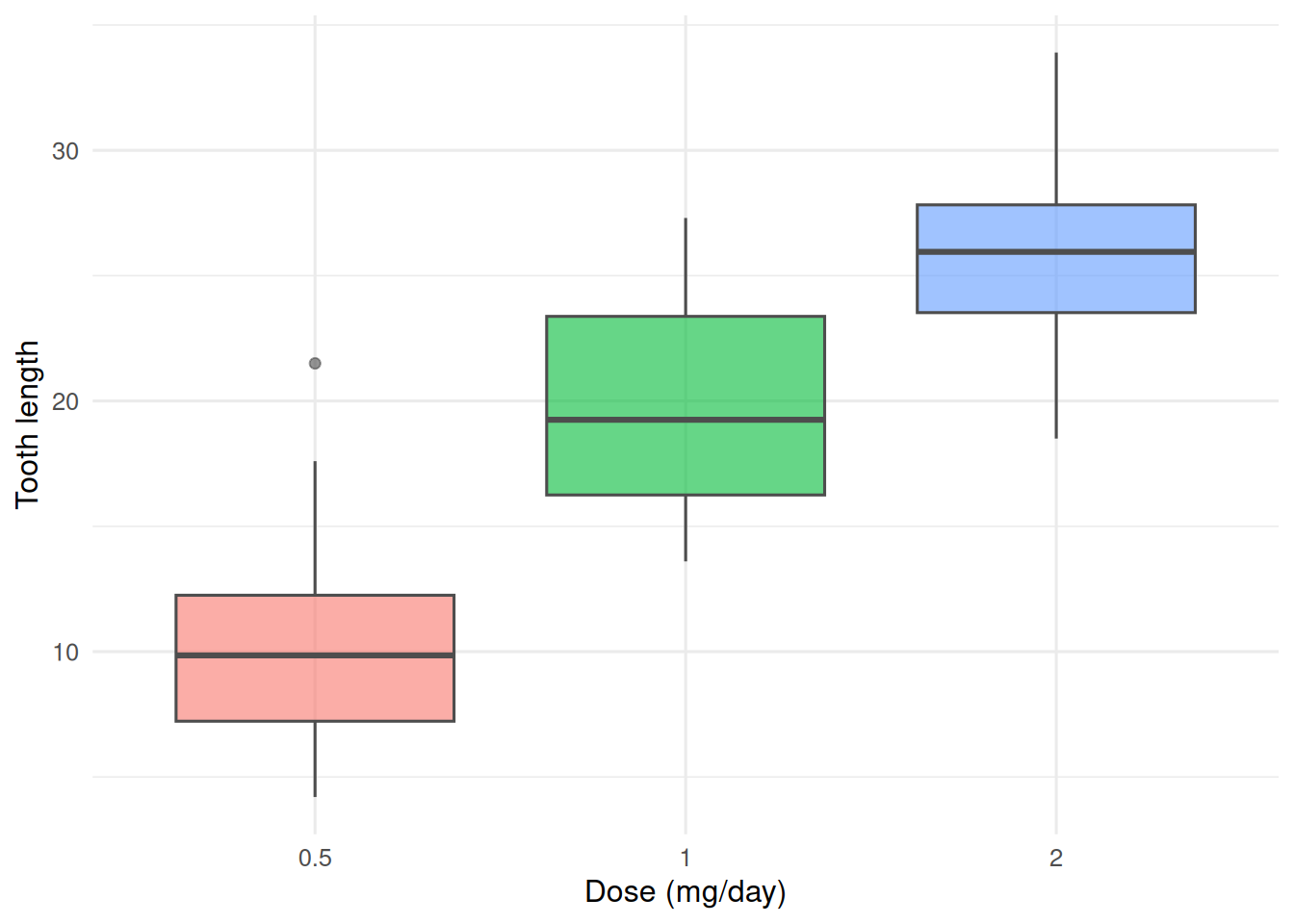
Using ToothGrowth, ask whether guinea-pig tooth length depends on dose of vitamin C.
Null: mean tooth length is equal across the three doses. Alternative: at least one dose differs.
2. Visualise
3. Assumptions
Approximate normality within groups and equal variances.
    Bartlett test of homogeneity of variances

data:  len by dose
Bartlett's K-squared = 0.66547, df = 2, p-value = 0.717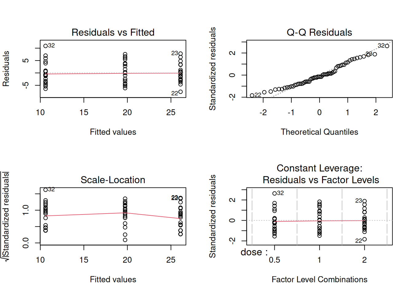
4. Conduct
            Df Sum Sq Mean Sq F value   Pr(>F)
dose         2   2426    1213   67.42 9.53e-16 ***
Residuals   57   1026      18
---
Signif. codes: 0 '***' 0.001 '**' 0.01 '*' 0.05 '.' 0.1 ' ' 1 dose emmean SE df lower.CL upper.CL
0.5 10.6 0.949 57 8.71 12.5
1 19.7 0.949 57 17.84 21.6
2 26.1 0.949 57 24.20 28.0
Confidence level used: 0.95 contrast estimate SE df t.ratio p.value
dose0.5 - dose1 -9.13 1.34 57 -6.806 <0.0001
dose0.5 - dose2 -15.49 1.34 57 -11.551 <0.0001
dose1 - dose2 -6.37 1.34 57 -4.745 <0.0001
P value adjustment: tukey method for comparing a family of 3 estimates 5. Concluding statement
Tooth length increased with dose of vitamin C (one-way ANOVA F = 67.42; p = 9.5^{-16}). Tukey-adjusted contrasts indicated that the 2 mg/day dose gave longer teeth than both lower doses (all adjusted p < 0.05).
Common pitfalls
- Stopping at a significant F without reporting which contrasts drive it.
- Reporting unadjusted pairwise p-values after the omnibus test.
- Treating a non-significant Bartlett test as proof of equal variances.
Further reading
- Lenth RV. emmeans package vignette.
- Oehlert GW. A First Course in Design and Analysis of Experiments.
- Maxwell SE, Delaney HD. Designing Experiments and Analyzing Data.
Session info
R version 4.5.2 (2025-10-31 ucrt)
Platform: x86_64-w64-mingw32/x64
Running under: Windows 11 x64 (build 26200)

Matrix products: default
  LAPACK version 3.12.1

locale:
[1] LC_COLLATE=English_Germany.utf8  LC_CTYPE=English_Germany.utf8
[3] LC_MONETARY=English_Germany.utf8 LC_NUMERIC=C
[5] LC_TIME=English_Germany.utf8

time zone: Europe/Berlin
tzcode source: internal

attached base packages:
[1] stats     graphics  grDevices utils     datasets  methods   base

other attached packages:
 [1] emmeans_2.0.3   broom_1.0.12    lubridate_1.9.5 forcats_1.0.1
 [5] stringr_1.6.0   dplyr_1.2.1     purrr_1.2.2     readr_2.2.0
 [9] tidyr_1.3.2     tibble_3.3.1    ggplot2_4.0.3   tidyverse_2.0.0

loaded via a namespace (and not attached):
 [1] sandwich_3.1-1     generics_0.1.4     stringi_1.8.7      lattice_0.22-9
 [5] hms_1.1.4          digest_0.6.39      magrittr_2.0.4     evaluate_1.0.5
 [9] grid_4.5.2         timechange_0.4.0   estimability_1.5.1 RColorBrewer_1.1-3
[13] mvtnorm_1.3-7      fastmap_1.2.0      Matrix_1.7-5       jsonlite_2.0.0
[17] backports_1.5.1    survival_3.8-6     multcomp_1.4-30    scales_1.4.0
[21] TH.data_1.1-5      codetools_0.2-20   cli_3.6.6          rlang_1.2.0
[25] splines_4.5.2      withr_3.0.2        yaml_2.3.12        otel_0.2.0
[29] tools_4.5.2        tzdb_0.5.0         coda_0.19-4.1      vctrs_0.7.3
[33] R6_2.6.1           zoo_1.8-15         lifecycle_1.0.5    htmlwidgets_1.6.4
[37] MASS_7.3-65        pkgconfig_2.0.3    pillar_1.11.1      gtable_0.3.6
[41] glue_1.8.1         xfun_0.57          tidyselect_1.2.1   knitr_1.51
[45] xtable_1.8-8       farver_2.1.2       htmltools_0.5.9    labeling_0.4.3
[49] rmarkdown_2.31     compiler_4.5.2     S7_0.2.2