Week 2, Session 5 — Non-linear regression with nls

Course 2 — #courses

R. Heller

Note

Inference labs use the five-step template: Hypothesis → Visualise → Assumptions → Conduct → Conclude.

Learning objectives

• Fit a parametric non-linear model with nls() and report the three parameters.
• Choose starting values that let the optimiser converge.
• Distinguish a GAM’s flexible curve from an nls model’s mechanistic curve.

Prerequisites

Sessions 2 and 4 of this week.

Background

Where a GAM says fit a smooth and see what shape it takes, nls says this curve has a known parametric form and I want the parameters. Michaelis–Menten kinetics, three-parameter logistic dose-response, and exponential decay are all examples of mechanistic models where the parameters have physical meanings: asymptote, half-maximal response, rate, and so on.

Fitting non-linear models is slightly more fragile than fitting linear ones because the optimiser must start somewhere and can get lost. Sensible starting values come from the shape of the data: the asymptote from the highest fitted values, the inflection from where the curve flattens, and so on. SSlogis and related self-starting functions estimate these automatically for common parameterisations.

nls gives asymptotic standard errors by default. For small samples or poor parameter identifiability, bootstrap or profile-likelihood intervals (confint(fit) uses profiles) are more honest.

Setup

library(tidyverse)
library(broom)
set.seed(42)
theme_set(theme_minimal(base_size = 12))

1. Hypothesis

Simulate dose-response data and fit a three-parameter logistic.

2. Visualise

n <- 60
dose <- rep(c(0.1, 0.3, 1, 3, 10, 30), each = 10)
# true params: asym = 100, xmid = log(3), scal = 0.7 (log-scale)
true_resp <- 100 / (1 + exp(-(log(dose) - log(3)) / 0.7))
resp <- true_resp + rnorm(n, 0, 5)
dat <- tibble(dose, resp)

ggplot(dat, aes(dose, resp)) +
  geom_point(alpha = 0.7) +
  scale_x_log10() +
  labs(x = "Dose (log scale)", y = "Response")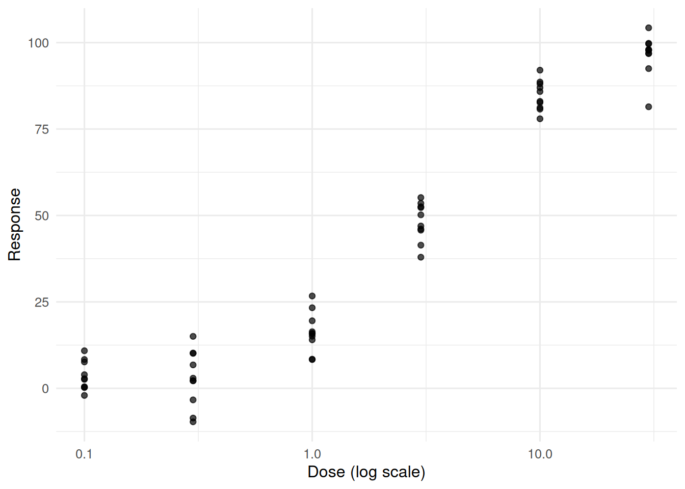

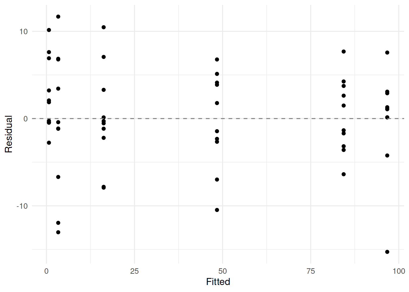
3. Assumptions

Correct model form, independent normal errors with constant variance on the response scale, and informative starting values.

fit <- nls(resp ~ SSlogis(log(dose), Asym, xmid, scal), data = dat)
resid_plot <- tibble(fitted = fitted(fit), resid = resid(fit))
ggplot(resid_plot, aes(fitted, resid)) +
  geom_point() +
  geom_hline(yintercept = 0, linetype = 2, colour = "grey50") +
  labs(x = "Fitted", y = "Residual")

4. Conduct

summary(fit)

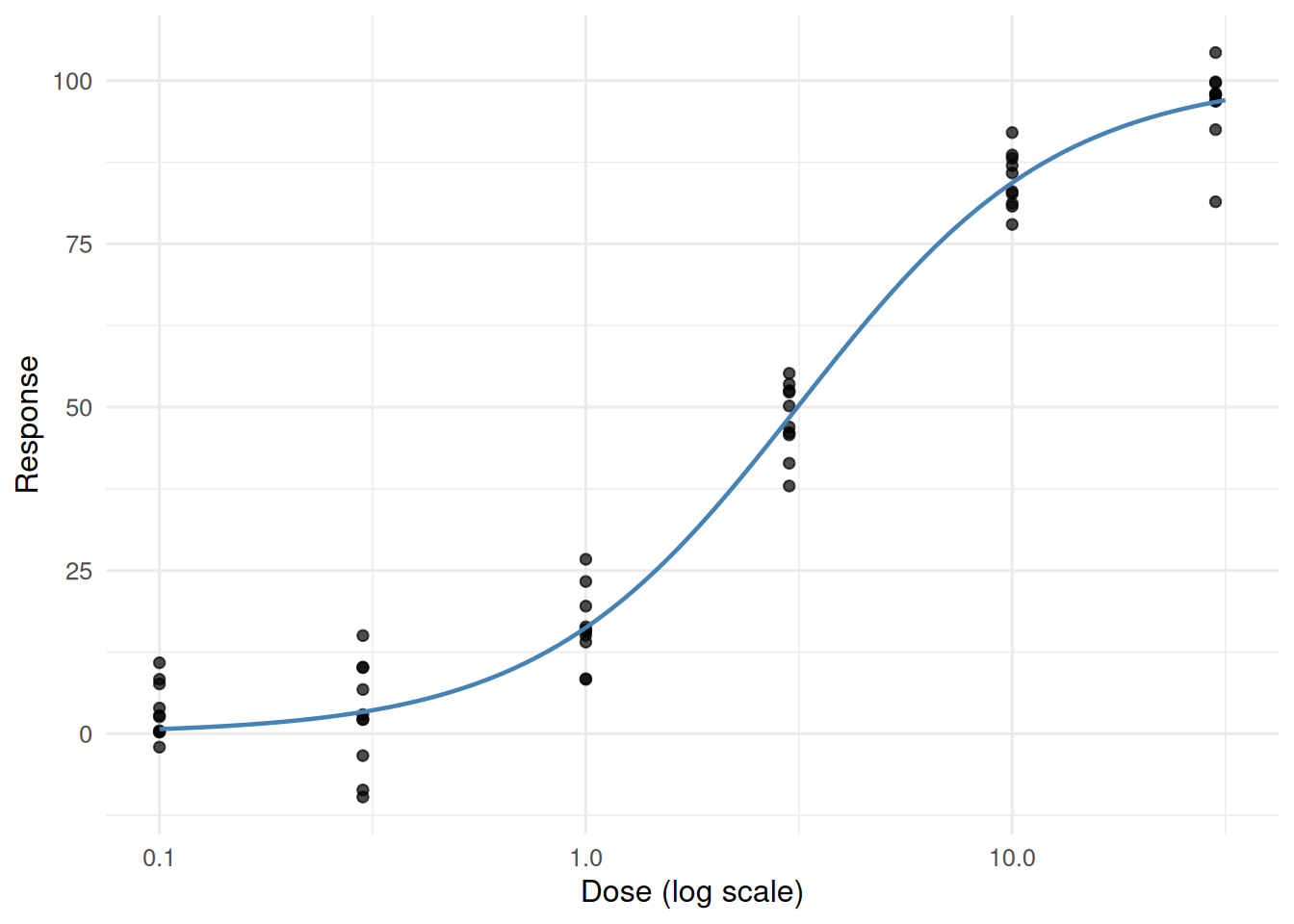
Formula: resp ~ SSlogis(log(dose), Asym, xmid, scal)

Parameters:
      Estimate Std. Error t value Pr(>|t|)    
Asym 100.58109    2.60639   38.59   <2e-16 ***
xmid   1.15107    0.06694   17.20   <2e-16 ***
scal   0.69868    0.05199   13.44   <2e-16 ***
---
Signif. codes:  0 '***' 0.001 '**' 0.01 '*' 0.05 '.' 0.1 ' ' 1

Residual standard error: 5.799 on 57 degrees of freedom

Number of iterations to convergence: 0 
Achieved convergence tolerance: 1.244e-07

confint(fit)

           2.5%       97.5%
Asym 95.7741920 106.3804894
xmid  1.0257176   1.2963776
scal  0.5989972   0.8113004

pred <- tibble(dose = 10 ^ seq(-1, 1.5, length.out = 100))
pred$resp <- predict(fit, newdata = pred)

ggplot(dat, aes(dose, resp)) +
  geom_point(alpha = 0.7) +
  geom_line(data = pred, colour = "steelblue", linewidth = 0.8) +
  scale_x_log10() +
  labs(x = "Dose (log scale)", y = "Response")

5. Concluding statement

A three-parameter logistic fitted on the log-dose scale returned an asymptote of 100.6 units and a mid-dose (EC50) at 3.16. Confidence intervals were obtained via the likelihood profile (see confint).

Explain why the self-starting function matters: without it, the student is confronted with finding starts for three parameters from scratch, which distracts from the concept.

Common pitfalls

• Starting values that put the optimiser in a local minimum.
• Reporting symmetric SE-based intervals when the likelihood is asymmetric; prefer confint.
• Over-interpreting parameters when the data do not span the asymptote.

Further reading

• Bates DM, Watts DG. Nonlinear Regression Analysis and Its Applications.
• Ritz C, Streibig JC. Nonlinear Regression with R.
• Pinheiro JC, Bates DM. Mixed-Effects Models in S and S-PLUS, ch. 8.

Session info

sessionInfo()

R version 4.4.1 (2024-06-14)
Platform: x86_64-pc-linux-gnu
Running under: Ubuntu 24.04.4 LTS

Matrix products: default
BLAS:   /usr/lib/x86_64-linux-gnu/openblas-pthread/libblas.so.3 
LAPACK: /usr/lib/x86_64-linux-gnu/openblas-pthread/libopenblasp-r0.3.26.so;  LAPACK version 3.12.0

locale:
 [1] LC_CTYPE=C.UTF-8       LC_NUMERIC=C           LC_TIME=C.UTF-8       
 [4] LC_COLLATE=C.UTF-8     LC_MONETARY=C.UTF-8    LC_MESSAGES=C.UTF-8   
 [7] LC_PAPER=C.UTF-8       LC_NAME=C              LC_ADDRESS=C          
[10] LC_TELEPHONE=C         LC_MEASUREMENT=C.UTF-8 LC_IDENTIFICATION=C   

time zone: UTC
tzcode source: system (glibc)

attached base packages:
[1] stats     graphics  grDevices utils     datasets  methods   base     

other attached packages:
 [1] broom_1.0.12    lubridate_1.9.5 forcats_1.0.1   stringr_1.6.0  
 [5] dplyr_1.2.1     purrr_1.2.2     readr_2.2.0     tidyr_1.3.2    
 [9] tibble_3.3.1    ggplot2_4.0.3   tidyverse_2.0.0

loaded via a namespace (and not attached):
 [1] gtable_0.3.6       jsonlite_2.0.0     compiler_4.4.1     tidyselect_1.2.1  
 [5] scales_1.4.0       yaml_2.3.12        fastmap_1.2.0      R6_2.6.1          
 [9] labeling_0.4.3     generics_0.1.4     knitr_1.51         backports_1.5.1   
[13] htmlwidgets_1.6.4  pillar_1.11.1      RColorBrewer_1.1-3 tzdb_0.5.0        
[17] rlang_1.2.0        stringi_1.8.7      xfun_0.57          S7_0.2.2          
[21] otel_0.2.0         timechange_0.4.0   cli_3.6.6          withr_3.0.2       
[25] magrittr_2.0.5     digest_0.6.39      grid_4.4.1         hms_1.1.4         
[29] lifecycle_1.0.5    vctrs_0.7.3        evaluate_1.0.5     glue_1.8.1        
[33] farver_2.1.2       rmarkdown_2.31     tools_4.4.1        pkgconfig_2.0.3   
[37] htmltools_0.5.9