Week 3, Session 1 — Logistic regression (binomial GLM)

Course 2 — #courses

R. Heller

Note

Inference labs use the five-step template: Hypothesis → Visualise → Assumptions → Conduct → Conclude.

Learning objectives

• Fit a logistic regression with glm(family = binomial) and translate coefficients into odds ratios.
• Construct a confusion matrix at a chosen probability threshold.
• Report the model with an odds ratio, an interval, and a brief note on discrimination.

Prerequisites

Week 1 regression material.

Background

Logistic regression models the log-odds of a binary outcome as a linear combination of predictors. The exponent of a coefficient is the odds ratio for a one-unit increase in the corresponding predictor. Because the relationship is linear on the log-odds scale and not the probability scale, a slope of 0.5 log-odds is a larger change in probability near 0.5 than near 0.95.

The model is fit by maximum likelihood with iteratively reweighted least squares. Standard errors are computed from the observed information, and Wald intervals on the log-odds scale are exponentiated to give intervals on the odds ratio. Profile-likelihood intervals are more trustworthy when the sample is small or the predictor is strongly associated with the outcome.

A confusion matrix at a single threshold tells only part of the story; the thresholds used in the clinic may not be the one that maximises accuracy. Week 3, Session 5 covers ROC curves and calibration, which give a threshold-free view of the same model.

Setup

library(tidyverse)
library(broom)
library(MASS)
set.seed(42)
theme_set(theme_minimal(base_size = 12))

1. Hypothesis

Using MASS::Pima.tr, can plasma glucose (glu) predict diabetes status (type)?

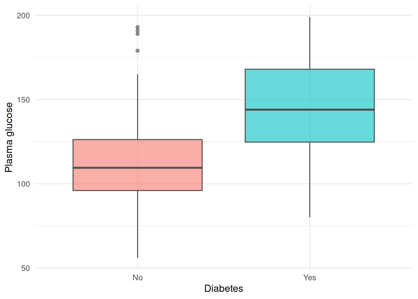
2. Visualise

pima <- as_tibble(Pima.tr) |>
  mutate(type = factor(type, levels = c("No", "Yes")))

ggplot(pima, aes(type, glu, fill = type)) +
  geom_boxplot(alpha = 0.6, colour = "grey30") +
  labs(x = "Diabetes", y = "Plasma glucose") +
  theme(legend.position = "none")

3. Assumptions

Binary outcome, independent observations, log-odds linear in the predictors (or handled explicitly with a smooth/transformation).

fit <- glm(type ~ glu, data = pima, family = binomial)
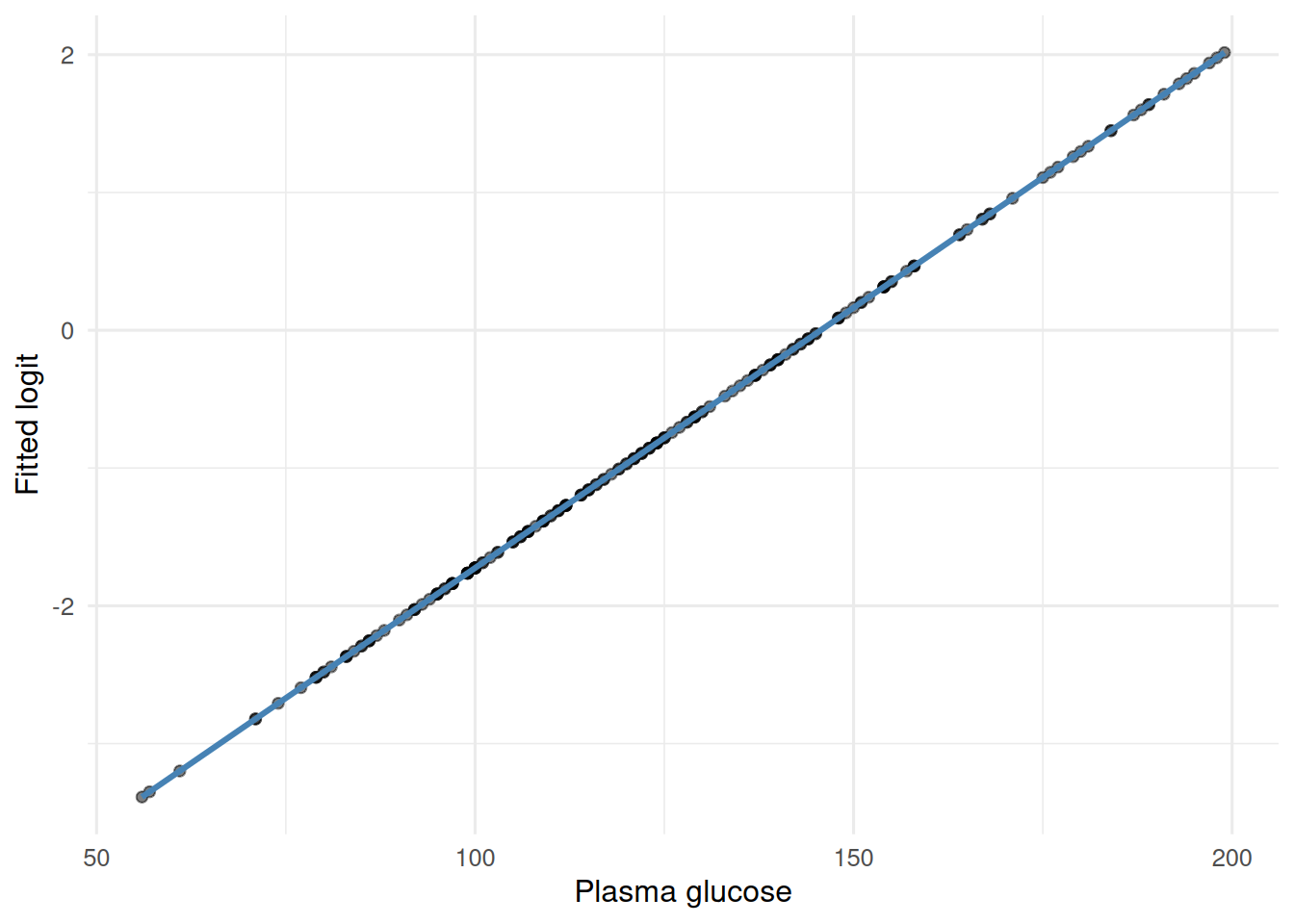
# residuals are less informative in GLMs; check for linearity on the logit scale
pima |>
  mutate(p = fitted(fit),
         logit = qlogis(p)) |>
  ggplot(aes(glu, logit)) +
  geom_point(alpha = 0.5) +
  geom_smooth(method = "loess", se = FALSE, colour = "steelblue") +
  labs(x = "Plasma glucose", y = "Fitted logit")

4. Conduct

tidy(fit, conf.int = TRUE, exponentiate = TRUE)

# A tibble: 2 × 7
  term        estimate std.error statistic  p.value conf.low conf.high
  <chr>          <dbl>     <dbl>     <dbl>    <dbl>    <dbl>     <dbl>
1 (Intercept)  0.00407   0.836       -6.58 4.62e-11 0.000714    0.0192
2 glu          1.04      0.00628      6.02 1.76e- 9 1.03        1.05  

glance(fit)

# A tibble: 1 × 8
  null.deviance df.null logLik   AIC   BIC deviance df.residual  nobs
          <dbl>   <int>  <dbl> <dbl> <dbl>    <dbl>       <int> <int>
1          256.     199  -104.  211.  218.     207.         198   200

pred_prob <- predict(fit, type = "response")
pred_class <- ifelse(pred_prob > 0.5, "Yes", "No")
table(pred_class, truth = pima$type)

          truth
pred_class  No Yes
       No  118  36
       Yes  14  32

5. Concluding statement

In 200 women, each 10 mg/dL increase in plasma glucose was associated with an odds ratio for diabetes of 1.46 (95% CI from profile: 1.3 to 1.66). At a 0.5 threshold the classifier had 75% accuracy; a threshold-free assessment appears in Week 3 Session 5.

Most readers prefer ORs reported per 10 units of a continuous predictor rather than per single unit; the per-unit OR sometimes looks implausibly close to 1.

Common pitfalls

• Reporting the coefficient on the log-odds scale without exponentiating.
• Confusing probability and odds.
• Evaluating the model with accuracy at one threshold and nothing else.

Further reading

• Hosmer DW, Lemeshow S. Applied Logistic Regression.
• Harrell FE. Regression Modeling Strategies, ch. 10.
• Gelman A, Hill J. Data Analysis Using Regression and Multilevel….

Session info

sessionInfo()

R version 4.4.1 (2024-06-14)
Platform: x86_64-pc-linux-gnu
Running under: Ubuntu 24.04.4 LTS

Matrix products: default
BLAS:   /usr/lib/x86_64-linux-gnu/openblas-pthread/libblas.so.3 
LAPACK: /usr/lib/x86_64-linux-gnu/openblas-pthread/libopenblasp-r0.3.26.so;  LAPACK version 3.12.0

locale:
 [1] LC_CTYPE=C.UTF-8       LC_NUMERIC=C           LC_TIME=C.UTF-8       
 [4] LC_COLLATE=C.UTF-8     LC_MONETARY=C.UTF-8    LC_MESSAGES=C.UTF-8   
 [7] LC_PAPER=C.UTF-8       LC_NAME=C              LC_ADDRESS=C          
[10] LC_TELEPHONE=C         LC_MEASUREMENT=C.UTF-8 LC_IDENTIFICATION=C   

time zone: UTC
tzcode source: system (glibc)

attached base packages:
[1] stats     graphics  grDevices utils     datasets  methods   base     

other attached packages:
 [1] MASS_7.3-60.2   broom_1.0.12    lubridate_1.9.5 forcats_1.0.1  
 [5] stringr_1.6.0   dplyr_1.2.1     purrr_1.2.2     readr_2.2.0    
 [9] tidyr_1.3.2     tibble_3.3.1    ggplot2_4.0.3   tidyverse_2.0.0

loaded via a namespace (and not attached):
 [1] Matrix_1.7-0       gtable_0.3.6       jsonlite_2.0.0     compiler_4.4.1    
 [5] tidyselect_1.2.1   splines_4.4.1      scales_1.4.0       yaml_2.3.12       
 [9] fastmap_1.2.0      lattice_0.22-6     R6_2.6.1           labeling_0.4.3    
[13] generics_0.1.4     knitr_1.51         backports_1.5.1    htmlwidgets_1.6.4 
[17] pillar_1.11.1      RColorBrewer_1.1-3 tzdb_0.5.0         rlang_1.2.0       
[21] utf8_1.2.6         stringi_1.8.7      xfun_0.57          S7_0.2.2          
[25] otel_0.2.0         timechange_0.4.0   cli_3.6.6          mgcv_1.9-1        
[29] withr_3.0.2        magrittr_2.0.5     digest_0.6.39      grid_4.4.1        
[33] hms_1.1.4          nlme_3.1-164       lifecycle_1.0.5    vctrs_0.7.3       
[37] evaluate_1.0.5     glue_1.8.1         farver_2.1.2       rmarkdown_2.31    
[41] tools_4.4.1        pkgconfig_2.0.3    htmltools_0.5.9