Week 3, Session 3 — Ordinal and multinomial regression

Course 2 — #courses

R. Heller

Note

Inference labs use the five-step template: Hypothesis → Visualise → Assumptions → Conduct → Conclude.

Learning objectives

• Fit a proportional-odds model with MASS::polr() and report a cumulative odds ratio.
• Fit a multinomial logistic regression with nnet::multinom() for an unordered outcome.
• Check the proportional-odds assumption and decide what to do when it fails.

Prerequisites

Week 3 Session 1 on binary logistic regression.

Background

Ordinal outcomes — pain scales, tumour stages, Likert items — carry more information than a dichotomised version and usually less than a continuous version. The proportional-odds model (polr) assumes the effect of each predictor is the same across all cumulative splits of the response; the single coefficient is the log cumulative odds ratio. Multinomial logistic regression makes no such constraint and fits a separate logit for each non-reference category.

The proportional-odds assumption is strong. A Brant test (in the brant package) or simply comparing the polr fit to a multinomial fit on deviance can detect violations. When it fails, options include a partial proportional-odds model, the multinomial model, or a continuation-ratio model.

Multinomial models are notoriously hungry for data: each non-reference category requires a full set of coefficients. Reporting should list all coefficient tables and a global test (likelihood ratio) rather than a single p-value.

Setup

library(tidyverse)
library(broom)
library(MASS)
library(nnet)
set.seed(42)
theme_set(theme_minimal(base_size = 12))

1. Hypothesis

Simulate an ordinal outcome (symptom severity in three levels) driven by a single continuous exposure, then contrast the ordinal and multinomial analyses.

2. Visualise

n <- 400
x <- rnorm(n)
eta <- 1.2 * x
# cumulative cutpoints
probs <- cbind(
  plogis(-0.5 - eta),
  plogis(1.0 - eta) - plogis(-0.5 - eta),
  1 - plogis(1.0 - eta)
)
y <- apply(probs, 1, function(p) sample(1:3, 1, prob = p))
dat <- tibble(x, y = factor(y, levels = 1:3,
                            labels = c("mild", "moderate", "severe"),
                            ordered = TRUE))

ggplot(dat, aes(y, x, fill = y)) +
  geom_boxplot(alpha = 0.6, colour = "grey30") +
  labs(x = "Severity", y = "Exposure x") +
  theme(legend.position = "none")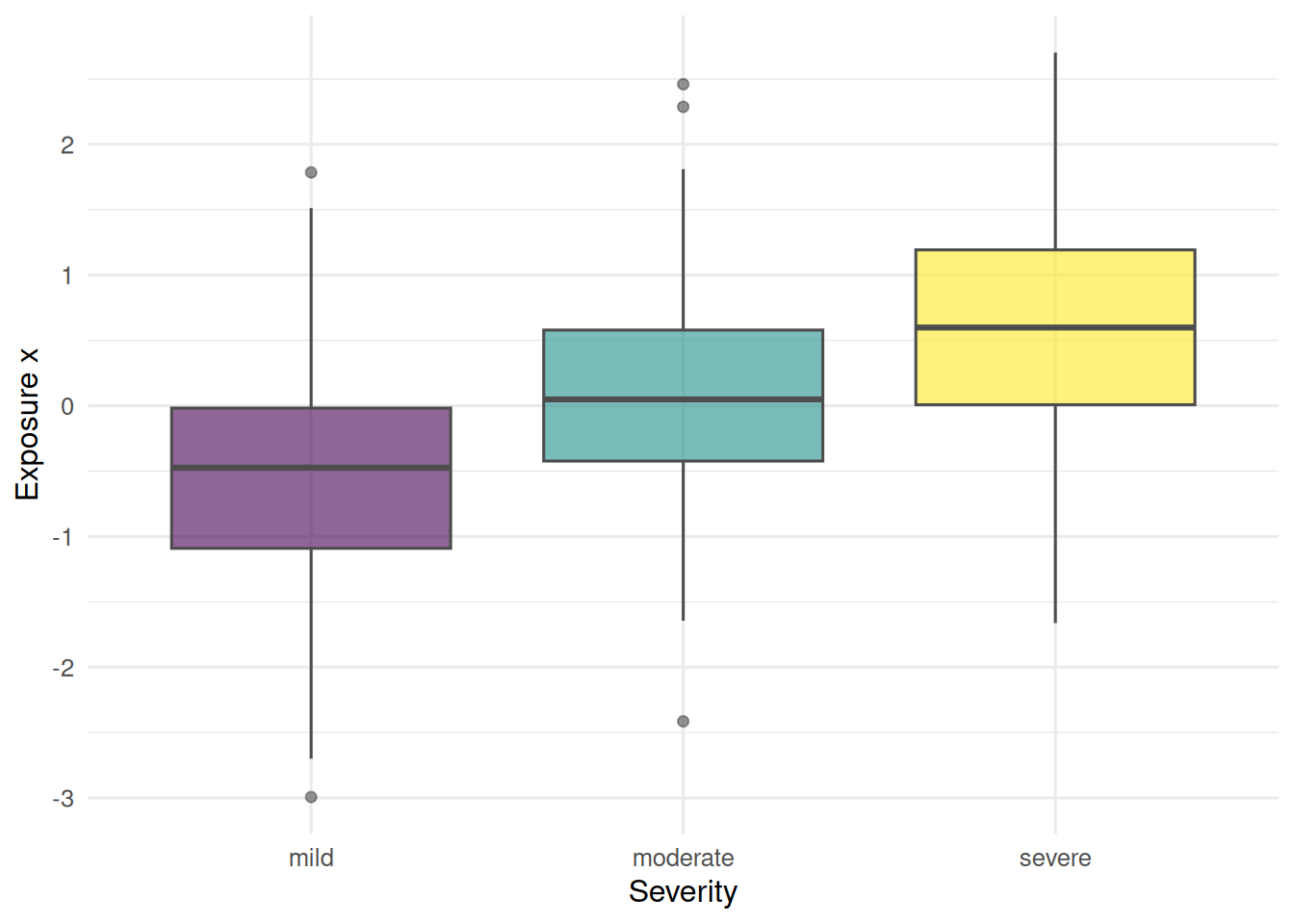

3. Assumptions

Proportional-odds (same β across cumulative splits) for polr; independent observations for both models.

# quick graphical check: fit logistic at each cumulative split and compare slopes
splits <- tibble(cut = c("mild vs rest", "mild+mod vs severe")) |>
  mutate(coef = c(
    coef(glm(I(as.numeric(y) >= 2) ~ x, data = dat, family = binomial))[2],
    coef(glm(I(as.numeric(y) >= 3) ~ x, data = dat, family = binomial))[2]
  ))
splits

# A tibble: 2 × 2
  cut                 coef
  <chr>              <dbl>
1 mild vs rest        1.18
2 mild+mod vs severe  1.16

If the two slopes are close, proportional odds is plausible.

4. Conduct

fit_polr <- polr(y ~ x, data = dat, Hess = TRUE)
summary(fit_polr)

Call:
polr(formula = y ~ x, data = dat, Hess = TRUE)

Coefficients:
  Value Std. Error t value
x 1.162     0.1249   9.297

Intercepts:
                Value   Std. Error t value
mild|moderate   -0.4652  0.1127    -4.1261
moderate|severe  0.9053  0.1198     7.5569

Residual Deviance: 757.0974 
AIC: 763.0974 

# approximate p-values
coef_summary <- coef(summary(fit_polr))
p <- pnorm(abs(coef_summary[, "t value"]), lower.tail = FALSE) * 2
cbind(coef_summary, "p value" = round(p, 3))

                     Value Std. Error   t value p value
x                1.1616521  0.1249448  9.297319       0
mild|moderate   -0.4651740  0.1127396 -4.126092       0
moderate|severe  0.9053007  0.1197974  7.556932       0

exp(coef(fit_polr))  # cumulative odds ratio

       x 
3.195208 

Multinomial:

fit_multi <- multinom(y ~ x, data = dat, trace = FALSE)
summary(fit_multi)

Call:
multinom(formula = y ~ x, data = dat, trace = FALSE)

Coefficients:
         (Intercept)         x
moderate  -0.2454994 0.8399669
severe    -0.2768431 1.5766088

Std. Errors:
         (Intercept)         x
moderate   0.1348679 0.1638624
severe     0.1417515 0.1815418

Residual Deviance: 756.7975 
AIC: 764.7975 

z <- summary(fit_multi)$coefficients / summary(fit_multi)$standard.errors
p_multi <- (1 - pnorm(abs(z), 0, 1)) * 2
round(p_multi, 3)

         (Intercept) x
moderate       0.069 0
severe         0.051 0

5. Concluding statement

The proportional-odds model returned a cumulative odds ratio per unit of x of 3.2, meaning larger x shifted symptom severity upward. The multinomial model returned two logits (moderate vs mild and severe vs mild) with effects in the same direction; deviance-based comparison did not reject the proportional-odds simplification.

A nice classroom moment: show both models side-by-side and note that polr spends one coefficient where multinom spends K − 1.

Common pitfalls

• Reporting only the odds ratio and ignoring whether proportional-odds holds.
• Using a multinomial model with a tiny reference category.
• Treating an ordered outcome as continuous and fitting a linear model.

Further reading

• Agresti A. Analysis of Ordinal Categorical Data.
• Harrell FE. Regression Modeling Strategies, ch. 13.
• Venables WN, Ripley BD. Modern Applied Statistics with S, ch. 7.

Session info

sessionInfo()

R version 4.4.1 (2024-06-14)
Platform: x86_64-pc-linux-gnu
Running under: Ubuntu 24.04.4 LTS

Matrix products: default
BLAS:   /usr/lib/x86_64-linux-gnu/openblas-pthread/libblas.so.3 
LAPACK: /usr/lib/x86_64-linux-gnu/openblas-pthread/libopenblasp-r0.3.26.so;  LAPACK version 3.12.0

locale:
 [1] LC_CTYPE=C.UTF-8       LC_NUMERIC=C           LC_TIME=C.UTF-8       
 [4] LC_COLLATE=C.UTF-8     LC_MONETARY=C.UTF-8    LC_MESSAGES=C.UTF-8   
 [7] LC_PAPER=C.UTF-8       LC_NAME=C              LC_ADDRESS=C          
[10] LC_TELEPHONE=C         LC_MEASUREMENT=C.UTF-8 LC_IDENTIFICATION=C   

time zone: UTC
tzcode source: system (glibc)

attached base packages:
[1] stats     graphics  grDevices utils     datasets  methods   base     

other attached packages:
 [1] nnet_7.3-19     MASS_7.3-60.2   broom_1.0.12    lubridate_1.9.5
 [5] forcats_1.0.1   stringr_1.6.0   dplyr_1.2.1     purrr_1.2.2    
 [9] readr_2.2.0     tidyr_1.3.2     tibble_3.3.1    ggplot2_4.0.3  
[13] tidyverse_2.0.0

loaded via a namespace (and not attached):
 [1] gtable_0.3.6       jsonlite_2.0.0     compiler_4.4.1     tidyselect_1.2.1  
 [5] scales_1.4.0       yaml_2.3.12        fastmap_1.2.0      R6_2.6.1          
 [9] labeling_0.4.3     generics_0.1.4     knitr_1.51         backports_1.5.1   
[13] htmlwidgets_1.6.4  pillar_1.11.1      RColorBrewer_1.1-3 tzdb_0.5.0        
[17] rlang_1.2.0        utf8_1.2.6         stringi_1.8.7      xfun_0.57         
[21] S7_0.2.2           otel_0.2.0         viridisLite_0.4.3  timechange_0.4.0  
[25] cli_3.6.6          withr_3.0.2        magrittr_2.0.5     digest_0.6.39     
[29] grid_4.4.1         hms_1.1.4          lifecycle_1.0.5    vctrs_0.7.3       
[33] evaluate_1.0.5     glue_1.8.1         farver_2.1.2       rmarkdown_2.31    
[37] tools_4.4.1        pkgconfig_2.0.3    htmltools_0.5.9