Week 3, Session 5 — Calibration, discrimination, ROC/AUC, Brier score

Course 2 — #courses

R. Heller

Note

Inference labs use the five-step template: Hypothesis → Visualise → Assumptions → Conduct → Conclude.

Learning objectives

• Separate discrimination (AUC) from calibration and from overall performance (Brier score).
• Draw an ROC curve with pROC and a calibration plot by binning predicted probabilities.
• Understand that a high AUC does not imply well-calibrated probabilities.

Prerequisites

Week 3 Session 1 on logistic regression.

Background

A risk prediction model should do three things well: separate events from non-events (discrimination), produce predicted probabilities that match observed frequencies (calibration), and balance both in a single summary of overall performance (the Brier score). A model can have high discrimination and poor calibration — for instance, if the predicted probabilities are systematically too extreme — and a model with perfect calibration can still be useless if it cannot separate cases from non-cases.

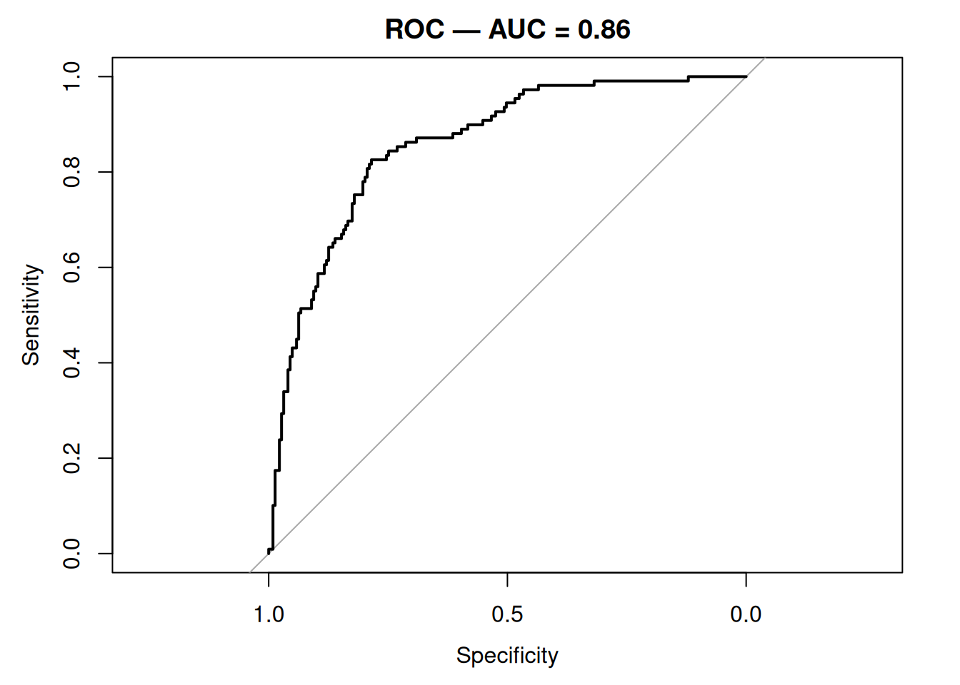
ROC analysis walks the decision threshold across all possible values and plots sensitivity against 1 − specificity. The area under the curve (AUC) is the probability that a randomly chosen case receives a higher predicted probability than a randomly chosen non-case. The Brier score is the mean squared error between predicted probabilities and the 0/1 outcome; a perfect model has a Brier of 0 and the no-skill model has Brier equal to the variance of the outcome.

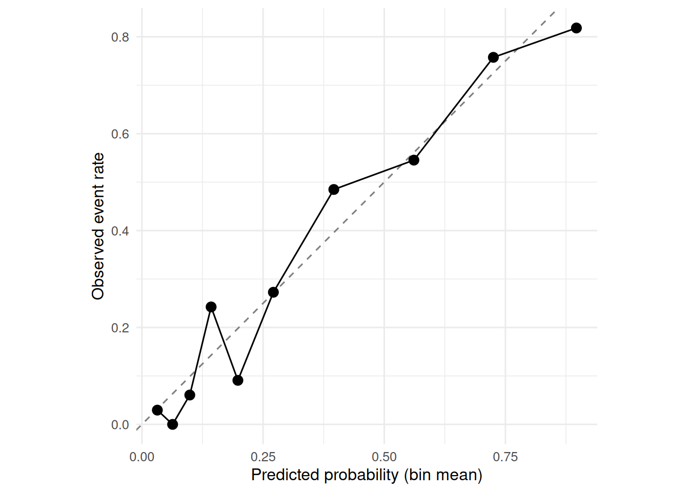
Calibration plots group predicted probabilities into bins and plot the observed event rate in each bin against the mean predicted probability. A 45° reference line is perfect calibration. Smoothed (LOESS) calibration curves are an alternative in larger samples.

Setup

library(tidyverse)
library(broom)
library(MASS)
library(pROC)
set.seed(42)
theme_set(theme_minimal(base_size = 12))

1. Hypothesis

Using MASS::Pima.tr (train) and MASS::Pima.te (test), fit a logistic regression and evaluate its discrimination, calibration, and Brier score.

2. Visualise

train <- as_tibble(Pima.tr) |> mutate(y = as.integer(type == "Yes"))
test  <- as_tibble(Pima.te) |> mutate(y = as.integer(type == "Yes"))

fit <- glm(y ~ glu + bmi + age + ped, data = train, family = binomial)
test$p <- predict(fit, test, type = "response")

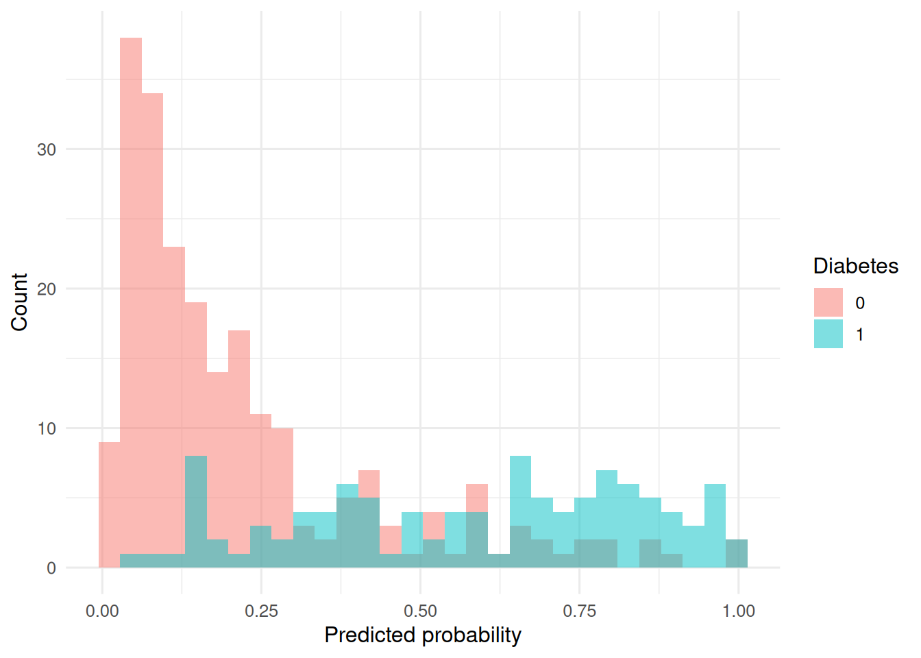
ggplot(test, aes(p, fill = factor(y))) +
  geom_histogram(position = "identity", alpha = 0.5, bins = 30) +
  labs(x = "Predicted probability", y = "Count", fill = "Diabetes")

3. Assumptions

The usual logistic-regression assumptions for the training fit; evaluation is on held-out data.

4. Conduct

Discrimination:

roc_obj <- roc(test$y, test$p, quiet = TRUE)
auc(roc_obj)

Area under the curve: 0.8585

ci.auc(roc_obj)

95% CI: 0.8173-0.8997 (DeLong)

plot(roc_obj, main = sprintf("ROC — AUC = %.2f", auc(roc_obj)))

Calibration (decile binning):

cal <- test |>
  mutate(bin = ntile(p, 10)) |>
  group_by(bin) |>
  summarise(predicted = mean(p), observed = mean(y), n = n())

ggplot(cal, aes(predicted, observed)) +
  geom_abline(linetype = 2, colour = "grey50") +
  geom_point(size = 3) +
  geom_line() +
  coord_equal() +
  labs(x = "Predicted probability (bin mean)",
       y = "Observed event rate")

Brier score:

brier <- mean((test$p - test$y)^2)
brier

[1] 0.1417249

5. Concluding statement

On the held-out test set (n = 332), the four-predictor logistic model achieved AUC = 0.86 (95% CI: 0.82 to 0.9) and a Brier score of 0.142. Calibration by decile was close to the 45° line.

Emphasise that AUC alone is a performance half-story. Clinicians using the predicted probability as a risk need calibration too.

Common pitfalls

• Reporting AUC on the training set without cross-validation.
• Using accuracy at a 0.5 threshold when the prevalence is not 0.5.
• Treating a single deciles-calibration plot as a formal test.

Further reading

• Steyerberg EW. Clinical Prediction Models.
• Harrell FE. Regression Modeling Strategies, ch. 10.
• Van Calster B et al. (2019), Calibration: the Achilles heel…

Session info

sessionInfo()

R version 4.5.2 (2025-10-31 ucrt)
Platform: x86_64-w64-mingw32/x64
Running under: Windows 11 x64 (build 26200)

Matrix products: default
  LAPACK version 3.12.1

locale:
[1] LC_COLLATE=English_Germany.utf8  LC_CTYPE=English_Germany.utf8   
[3] LC_MONETARY=English_Germany.utf8 LC_NUMERIC=C                    
[5] LC_TIME=English_Germany.utf8    

time zone: Europe/Berlin
tzcode source: internal

attached base packages:
[1] stats     graphics  grDevices utils     datasets  methods   base     

other attached packages:
 [1] pROC_1.19.0.1   MASS_7.3-65     broom_1.0.12    lubridate_1.9.5
 [5] forcats_1.0.1   stringr_1.6.0   dplyr_1.2.1     purrr_1.2.2    
 [9] readr_2.2.0     tidyr_1.3.2     tibble_3.3.1    ggplot2_4.0.3  
[13] tidyverse_2.0.0

loaded via a namespace (and not attached):
 [1] gtable_0.3.6       jsonlite_2.0.0     compiler_4.5.2     Rcpp_1.1.1-1.1    
 [5] tidyselect_1.2.1   scales_1.4.0       yaml_2.3.12        fastmap_1.2.0     
 [9] R6_2.6.1           labeling_0.4.3     generics_0.1.4     knitr_1.51        
[13] backports_1.5.1    htmlwidgets_1.6.4  pillar_1.11.1      RColorBrewer_1.1-3
[17] tzdb_0.5.0         rlang_1.2.0        stringi_1.8.7      xfun_0.57         
[21] S7_0.2.2           otel_0.2.0         timechange_0.4.0   cli_3.6.6         
[25] withr_3.0.2        magrittr_2.0.4     digest_0.6.39      grid_4.5.2        
[29] hms_1.1.4          lifecycle_1.0.5    vctrs_0.7.3        evaluate_1.0.5    
[33] glue_1.8.1         farver_2.1.2       rmarkdown_2.31     tools_4.5.2       
[37] pkgconfig_2.0.3    htmltools_0.5.9