Week 4, Session 2 — Kappa, ICC, Bland–Altman

Course 2 — #courses

R. Heller

Note

Workflow labs use the variant template: Goal → Approach → Execution → Check → Report.

Learning objectives

• Compute Cohen’s kappa for categorical agreement and explain its chance-correction.
• Compute an intraclass correlation coefficient for continuous agreement and distinguish consistency from absolute agreement.
• Draw a Bland–Altman plot and report limits of agreement.

Prerequisites

Basic R and ggplot2.

Background

Measurement-agreement studies ask whether two raters, two methods, or two instruments give the same answer on the same units. The choice of statistic depends on the scale of the measurement. Cohen’s kappa adjusts simple percent agreement for the agreement expected by chance given the marginal frequencies; it ranges from −1 to 1 with common landmarks at 0.4 and 0.6. Its main weakness is sensitivity to prevalence.

For continuous measurements, the intraclass correlation (ICC) and the Bland–Altman plot answer complementary questions. The ICC is a single-number summary of reliability, defined in several flavours (one-way, two-way, consistency vs absolute). The Bland–Altman plot shows pattern: it plots the difference between two raters against their mean and marks the limits of agreement (typically mean ± 1.96 SD). It reveals bias, proportional bias, and heteroscedasticity that ICCs hide.

Reliability is not the same as agreement. Two raters can be highly correlated (one is always twice the other) and have a terrible agreement. Always report both and let the picture tell the pattern.

Setup

library(tidyverse)
library(broom)
library(psych)
library(irr)
set.seed(42)
theme_set(theme_minimal(base_size = 12))

1. Goal

Build two small rater datasets — one categorical, one continuous — and compute the matching agreement statistics.

2. Approach

For the categorical example, simulate 100 radiograph classifications (3 categories) by two readers with substantial but not perfect agreement. For the continuous example, simulate 60 measurements by two instruments, one with a small constant bias.

# categorical
cats <- c("normal", "mild", "severe")
truth <- sample(cats, 100, replace = TRUE, prob = c(0.5, 0.3, 0.2))
r1 <- ifelse(runif(100) < 0.2, sample(cats, 100, replace = TRUE), truth)
r2 <- ifelse(runif(100) < 0.25, sample(cats, 100, replace = TRUE), truth)
kap_tbl <- tibble(r1 = factor(r1, levels = cats),
                  r2 = factor(r2, levels = cats))

# continuous
n <- 60
true_val <- rnorm(n, 100, 15)
inst1 <- true_val + rnorm(n, 0, 3)
inst2 <- true_val + 2 + rnorm(n, 0, 3)    # small positive bias
meas <- tibble(inst1, inst2)

3. Execution

Cohen’s kappa:

kappa2(kap_tbl[, c("r1", "r2")])

 Cohen's Kappa for 2 Raters (Weights: unweighted)

 Subjects = 100 
   Raters = 2 
    Kappa = 0.584 

        z = 8.21 
  p-value = 2.22e-16 

ICC via psych:

ICC(as.matrix(meas))

Call: ICC(x = as.matrix(meas))

Intraclass correlation coefficients 
                         type  ICC  F df1 df2       p lower bound upper bound
Single_raters_absolute   ICC1 0.95 43  59  60 1.4e-33        0.93        0.97
Single_random_raters     ICC2 0.95 44  59  59 2.1e-33        0.93        0.97
Single_fixed_raters      ICC3 0.96 44  59  59 2.1e-33        0.93        0.97
Average_raters_absolute ICC1k 0.98 43  59  60 1.4e-33        0.96        0.99
Average_random_raters   ICC2k 0.98 44  59  59 2.1e-33        0.96        0.99
Average_fixed_raters    ICC3k 0.98 44  59  59 2.1e-33        0.96        0.99

 Number of subjects = 60     Number of Judges =  2
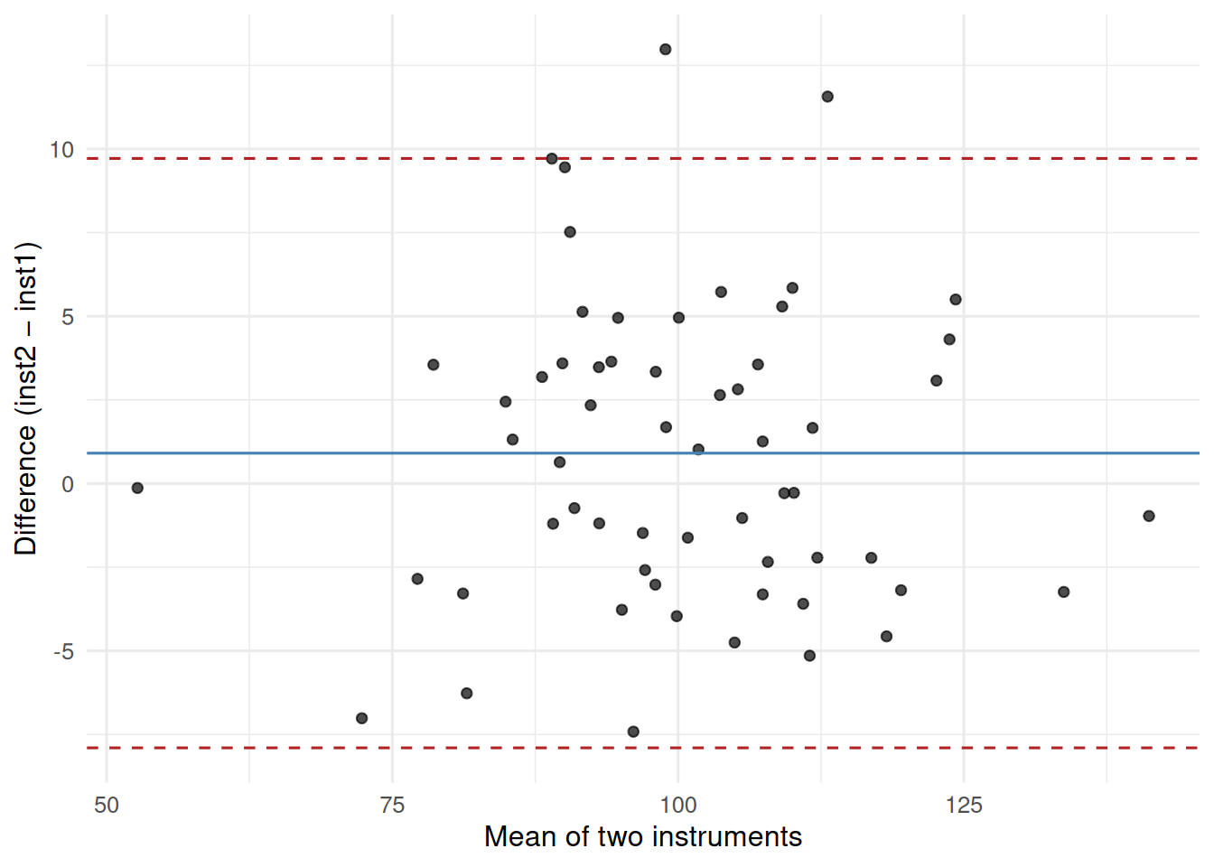
See the help file for a discussion of the other 4 McGraw and Wong estimates,

Bland–Altman:

ba <- meas |>
  mutate(mean_val = (inst1 + inst2) / 2,
         diff_val = inst2 - inst1)
loa <- mean(ba$diff_val) + c(-1.96, 0, 1.96) * sd(ba$diff_val)

ggplot(ba, aes(mean_val, diff_val)) +
  geom_point(alpha = 0.7) +
  geom_hline(yintercept = loa[1], linetype = 2, colour = "firebrick") +
  geom_hline(yintercept = loa[2], linetype = 1, colour = "steelblue") +
  geom_hline(yintercept = loa[3], linetype = 2, colour = "firebrick") +
  labs(x = "Mean of two instruments",
       y = "Difference (inst2 − inst1)")

4. Check

The ICC should be high (> 0.9) because the raters are well correlated, but the Bland–Altman plot shows a small positive bias (inst2 reads about 2 units higher on average).

5. Report

Cohen’s kappa for the two radiograph readers was 0.58. For the two instruments, the ICC (absolute agreement, two-way random) was 0.95, but the Bland–Altman plot revealed a mean bias of 0.9 units with 95% limits of agreement from -7.9 to 9.7.

Two takeaways: bias and precision are separate components of agreement, and neither kappa nor a single correlation captures both.

Common pitfalls

• Reporting percent agreement instead of kappa.
• Using Pearson r on two raters and calling it agreement.
• Omitting the limits of agreement from a Bland–Altman plot.

Further reading

• Bland JM, Altman DG (1986), Statistical methods for assessing agreement…
• Shrout PE, Fleiss JL (1979), Intraclass correlations…
• McGraw KO, Wong SP (1996), Forming inferences about some ICCs.

Session info

sessionInfo()

R version 4.4.1 (2024-06-14)
Platform: x86_64-pc-linux-gnu
Running under: Ubuntu 24.04.4 LTS

Matrix products: default
BLAS:   /usr/lib/x86_64-linux-gnu/openblas-pthread/libblas.so.3 
LAPACK: /usr/lib/x86_64-linux-gnu/openblas-pthread/libopenblasp-r0.3.26.so;  LAPACK version 3.12.0

locale:
 [1] LC_CTYPE=C.UTF-8       LC_NUMERIC=C           LC_TIME=C.UTF-8       
 [4] LC_COLLATE=C.UTF-8     LC_MONETARY=C.UTF-8    LC_MESSAGES=C.UTF-8   
 [7] LC_PAPER=C.UTF-8       LC_NAME=C              LC_ADDRESS=C          
[10] LC_TELEPHONE=C         LC_MEASUREMENT=C.UTF-8 LC_IDENTIFICATION=C   

time zone: UTC
tzcode source: system (glibc)

attached base packages:
[1] stats     graphics  grDevices utils     datasets  methods   base     

other attached packages:
 [1] irr_0.84.1      lpSolve_5.6.23  psych_2.6.3     broom_1.0.12   
 [5] lubridate_1.9.5 forcats_1.0.1   stringr_1.6.0   dplyr_1.2.1    
 [9] purrr_1.2.2     readr_2.2.0     tidyr_1.3.2     tibble_3.3.1   
[13] ggplot2_4.0.3   tidyverse_2.0.0

loaded via a namespace (and not attached):
 [1] generics_0.1.4     stringi_1.8.7      lattice_0.22-6     lme4_2.0-1        
 [5] hms_1.1.4          digest_0.6.39      magrittr_2.0.5     evaluate_1.0.5    
 [9] grid_4.4.1         timechange_0.4.0   RColorBrewer_1.1-3 fastmap_1.2.0     
[13] Matrix_1.7-0       jsonlite_2.0.0     backports_1.5.1    scales_1.4.0      
[17] reformulas_0.4.4   Rdpack_2.6.6       mnormt_2.1.2       cli_3.6.6         
[21] rlang_1.2.0        rbibutils_2.4.1    splines_4.4.1      withr_3.0.2       
[25] yaml_2.3.12        otel_0.2.0         tools_4.4.1        parallel_4.4.1    
[29] tzdb_0.5.0         nloptr_2.2.1       minqa_1.2.8        boot_1.3-30       
[33] vctrs_0.7.3        R6_2.6.1           lifecycle_1.0.5    htmlwidgets_1.6.4 
[37] MASS_7.3-60.2      pkgconfig_2.0.3    pillar_1.11.1      gtable_0.3.6      
[41] Rcpp_1.1.1-1.1     glue_1.8.1         xfun_0.57          tidyselect_1.2.1  
[45] knitr_1.51         farver_2.1.2       htmltools_0.5.9    nlme_3.1-164      
[49] labeling_0.4.3     rmarkdown_2.31     compiler_4.4.1     S7_0.2.2