Week 1, Session 1 — Observational designs and STROBE

Course 3 — #courses

R. Heller

Note

Workflow lab using the variant template: Goal → Approach → Execution → Check → Report.

Learning objectives

Distinguish cohort, case-control, and cross-sectional designs and say when each is the right tool.
Simulate a source population and draw both a cohort sample and a nested case-control sample from it.
Map a study report to the STROBE checklist.

Prerequisites

Course 1 (inference) and Course 2 (regression). Familiarity with tibbles and glm().

Background

Observational designs differ primarily in how participants enter the study and when the outcome is measured relative to the exposure. In a cohort we sample on exposure and wait; in a case-control we sample on the outcome and look back; in a cross-sectional we sample once and measure everything together. The choice is driven by how common the outcome is, how long it takes to develop, and how easy the exposure is to measure retrospectively.

STROBE (Strengthening the Reporting of Observational Studies in Epidemiology) is the reporting checklist that keeps observational papers honest. It has 22 items covering title and abstract, introduction, methods, results, and discussion, with specific branches for the three main designs. You do not need to memorise it; you need to know that reviewers will check it.

A nested case-control sampled from a defined cohort behaves statistically like the full cohort for odds ratios that approximate risk ratios when the outcome is rare. This is the trick behind most large pharmacoepidemiology studies: a full-cohort analysis is wasteful when measurement on every unexposed person is expensive, so analysts sample controls from the risk set instead.

Setup

library(tidyverse)
set.seed(42)
theme_set(theme_minimal(base_size = 12))

1. Goal

Simulate a source population, carve a cohort study and a nested case-control study out of it, and compare the exposure–outcome association recovered by each.

2. Approach

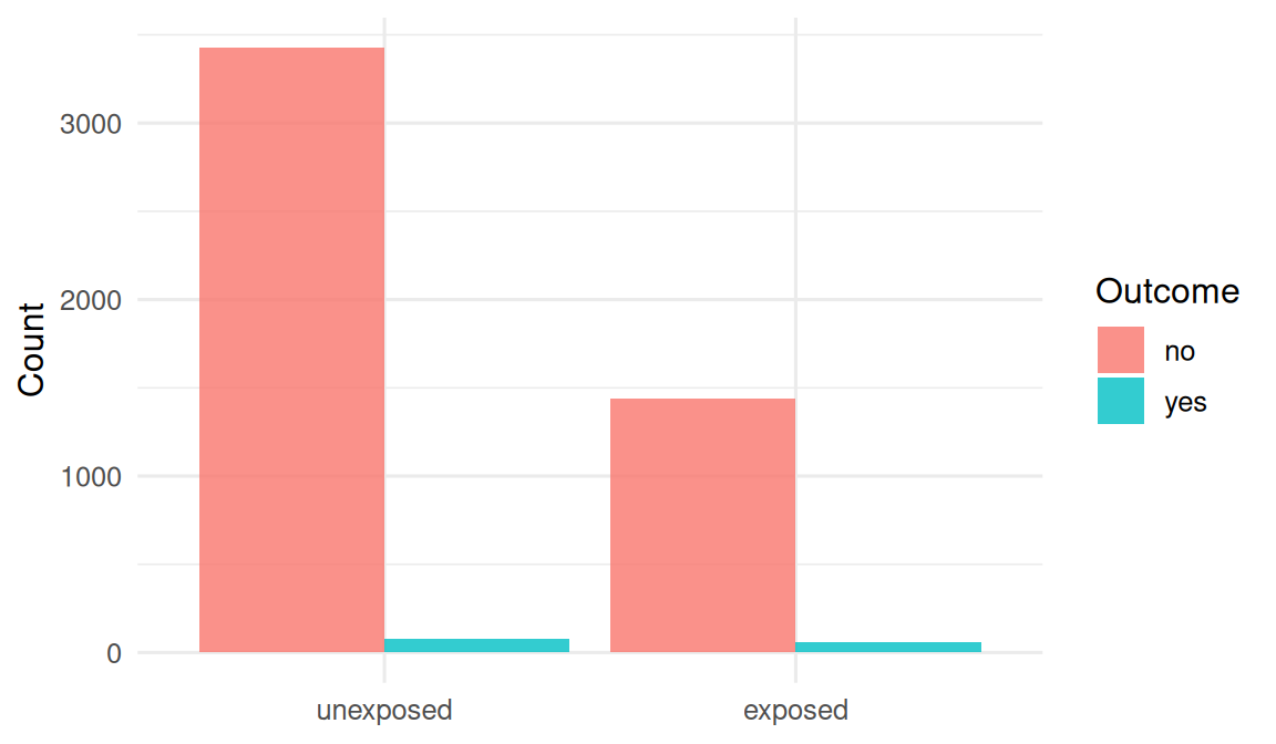
We generate a population of 5000 people with a binary exposure and a binary outcome whose probability depends on exposure and a confounder (age). We then (a) analyse the full cohort and (b) draw a case-control sample with four controls per case.

n_pop <- 5000
pop <- tibble(
  id       = seq_len(n_pop),
  age      = rnorm(n_pop, 55, 10),
  exposure = rbinom(n_pop, 1, 0.30)
)
# outcome depends on exposure (log OR ~ 0.8) and age
lp <- -4 + 0.8 * pop$exposure + 0.04 * (pop$age - 55)
pop <- pop |>
  mutate(prob = plogis(lp),
         outcome = rbinom(n_pop, 1, prob))

pop |>
  count(exposure, outcome) |>
  mutate(exposure = factor(exposure, labels = c("unexposed", "exposed")),
         outcome  = factor(outcome,  labels = c("no", "yes"))) |>
  ggplot(aes(exposure, n, fill = outcome)) +
  geom_col(position = "dodge", alpha = 0.8) +
  labs(x = NULL, y = "Count", fill = "Outcome")

3. Execution

# Cohort analysis on full population
fit_cohort <- glm(outcome ~ exposure + age, data = pop, family = binomial)
coef_cohort <- broom::tidy(fit_cohort, conf.int = TRUE, exponentiate = TRUE)
coef_cohort

# A tibble: 3 × 7
  term        estimate std.error statistic  p.value conf.low conf.high
  <chr>          <dbl>     <dbl>     <dbl>    <dbl>    <dbl>     <dbl>
1 (Intercept)  0.00361   0.512      -11.0  4.75e-28  0.00130   0.00972
2 exposure     1.92      0.174        3.75 1.74e- 4  1.36      2.71   
3 age          1.03      0.00863      3.74 1.87e- 4  1.02      1.05

# Nested case-control: all cases, 4 controls per case
cases    <- pop |> filter(outcome == 1)
controls <- pop |>
  filter(outcome == 0) |>
  slice_sample(n = 4 * nrow(cases))
ncc <- bind_rows(cases, controls)
fit_ncc <- glm(outcome ~ exposure + age, data = ncc, family = binomial)
coef_ncc <- broom::tidy(fit_ncc, conf.int = TRUE, exponentiate = TRUE)
coef_ncc

# A tibble: 3 × 7
  term        estimate std.error statistic       p.value conf.low conf.high
  <chr>          <dbl>     <dbl>     <dbl>         <dbl>    <dbl>     <dbl>
1 (Intercept)   0.0347   0.565       -5.95 0.00000000263   0.0112     0.103
2 exposure      2.10     0.197        3.76 0.000168        1.43       3.09 
3 age           1.03     0.00954      3.16 0.00156         1.01       1.05

4. Check

The exposure odds ratio from the nested case-control should be close to that from the cohort, because the outcome is uncommon. Precision is worse in the case-control sample but the point estimate is not biased by the sampling scheme.

bind_rows(
  cohort = coef_cohort |> filter(term == "exposure"),
  ncc    = coef_ncc    |> filter(term == "exposure"),
  .id = "design"
) |>
  select(design, estimate, conf.low, conf.high)

# A tibble: 2 × 4
  design estimate conf.low conf.high
  <chr>     <dbl>    <dbl>     <dbl>
1 cohort     1.92     1.36      2.71
2 ncc        2.10     1.43      3.09

5. Report

In a simulated source population of 5000 adults, exposure was associated with the outcome with an adjusted odds ratio of 1.92 (95% CI: 1.36 to 2.71) in a full-cohort analysis, and 2.1 (95% CI: 1.43 to 3.09) in a 1:4 nested case-control sample.

STROBE in one paragraph

Report the sampling frame, the eligibility criteria, the exposure and outcome definitions, how confounders were chosen and handled, whatever you did about missing data, and a flow diagram of who was included, excluded, and lost. If you can do those six things clearly, you have answered most of the STROBE items for free.

Common pitfalls

Treating a cross-sectional association as evidence of a causal effect when temporality is unknown.
Reporting an odds ratio as a risk ratio when the outcome is common.
Drawing controls from a different population than the cases.
Skipping a flow diagram in an observational paper.

Session info

sessionInfo()

R version 4.4.1 (2024-06-14)
Platform: x86_64-pc-linux-gnu
Running under: Ubuntu 24.04.4 LTS

Matrix products: default
BLAS:   /usr/lib/x86_64-linux-gnu/openblas-pthread/libblas.so.3 
LAPACK: /usr/lib/x86_64-linux-gnu/openblas-pthread/libopenblasp-r0.3.26.so;  LAPACK version 3.12.0

locale:
 [1] LC_CTYPE=C.UTF-8       LC_NUMERIC=C           LC_TIME=C.UTF-8       
 [4] LC_COLLATE=C.UTF-8     LC_MONETARY=C.UTF-8    LC_MESSAGES=C.UTF-8   
 [7] LC_PAPER=C.UTF-8       LC_NAME=C              LC_ADDRESS=C          
[10] LC_TELEPHONE=C         LC_MEASUREMENT=C.UTF-8 LC_IDENTIFICATION=C   

time zone: UTC
tzcode source: system (glibc)

attached base packages:
[1] stats     graphics  grDevices utils     datasets  methods   base     

other attached packages:
 [1] lubridate_1.9.5 forcats_1.0.1   stringr_1.6.0   dplyr_1.2.1    
 [5] purrr_1.2.2     readr_2.2.0     tidyr_1.3.2     tibble_3.3.1   
 [9] ggplot2_4.0.3   tidyverse_2.0.0

loaded via a namespace (and not attached):
 [1] gtable_0.3.6       jsonlite_2.0.0     compiler_4.4.1     tidyselect_1.2.1  
 [5] scales_1.4.0       yaml_2.3.12        fastmap_1.2.0      R6_2.6.1          
 [9] labeling_0.4.3     generics_0.1.4     knitr_1.51         backports_1.5.1   
[13] htmlwidgets_1.6.4  pillar_1.11.1      RColorBrewer_1.1-3 tzdb_0.5.0        
[17] rlang_1.2.0        utf8_1.2.6         broom_1.0.12       stringi_1.8.7     
[21] xfun_0.57          S7_0.2.2           otel_0.2.0         timechange_0.4.0  
[25] cli_3.6.6          withr_3.0.2        magrittr_2.0.5     digest_0.6.39     
[29] grid_4.4.1         hms_1.1.4          lifecycle_1.0.5    vctrs_0.7.3       
[33] evaluate_1.0.5     glue_1.8.1         farver_2.1.2       rmarkdown_2.31    
[37] tools_4.4.1        pkgconfig_2.0.3    htmltools_0.5.9

Week 1, Session 1 — Observational designs and STROBE

Learning objectives

Prerequisites

Background

Setup

1. Goal

2. Approach

3. Execution

4. Check

5. Report

STROBE in one paragraph

Common pitfalls

Further reading

Session info