Week 1, Session 5 — Power: closed-form and simulation
Course 3 — #courses
Note
Inference lab using the five-step template: Hypothesis → Visualise → Assumptions → Conduct → Conclude.
Learning objectives
- Run a closed-form power calculation for a two-sample t-test with
pwr. - Simulate power for a scenario where closed-form solutions do not exist using
simr. - Describe the inputs to any power calculation (effect, variance, alpha, design).
Prerequisites
Course 1 inference and Course 2 mixed-model basics (we will fit a small lmer).
Background
Power is the probability of rejecting the null hypothesis when a specific alternative is true. Four inputs set it: the effect size you care about, the variability of the outcome, the significance level, and the sample size (with the design). Closed-form formulas exist for standard one- and two-sample tests and for some simple regression settings. For anything more elaborate — clustered data, non-linear models, interim looks, complex survival designs — you simulate.
Simulation-based power is conceptually straightforward: for a given scenario, generate many datasets under the alternative, run the planned analysis on each, and compute the fraction of times you reject the null. The simr package does this for models fit with lme4, allowing you to vary the sample size or the effect and trace out a power curve.
A useful rule of thumb: if your closed-form calculation is for a model simpler than the one you will actually fit, the closed-form is giving you a lower bound on the sample size you need, not an answer.
Setup
1. Hypothesis
Detect a standardised mean difference of d = 0.4 between two groups with 80% power at a 5% two-sided significance level. Then power a mixed model with 20 clusters and 10 observations each to detect a fixed effect of 0.3.
2. Visualise
ns <- seq(20, 400, by = 20)
pw <- map_dbl(ns, \(n) pwr.t.test(
  n = n / 2, d = 0.4, sig.level = 0.05, type = "two.sample"
)$power)

tibble(n = ns, power = pw) |>
  ggplot(aes(n, power)) +
  geom_line() +
  geom_hline(yintercept = 0.8, linetype = "dashed", colour = "grey40") +
  labs(x = "Total sample size", y = "Power")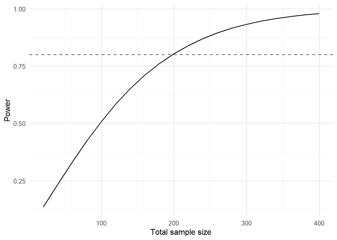
3. Assumptions
Closed-form assumes equal variance across arms, independent observations, and the nominal effect size. The simulation below adds random intercepts at the cluster level and therefore relaxes independence.
4. Conduct
     Two-sample t test power calculation

              n = 99.08032
              d = 0.4
      sig.level = 0.05
          power = 0.8
    alternative = two.sided

NOTE: n is number in *each* group
# Simulation: a small two-arm cluster study
J <- 20 # clusters
nj <- 10 # obs per cluster
dat <- tibble(
cluster = factor(rep(seq_len(J), each = nj)),
arm = rep(rep(c(0, 1), each = nj), length.out = J * nj),
y = rnorm(J * nj) # placeholder; simr overwrites
)
m0 <- makeLmer(
y ~ arm + (1 | cluster),
fixef = c(0, 0.3),
VarCorr = 0.5,
sigma = 1.0,
data = dat
)
m0Linear mixed model fit by REML ['lmerMod']
Formula: y ~ arm + (1 | cluster)
Data: dat
REML criterion at convergence: 576.9954
Random effects:
Groups Name Std.Dev.
cluster (Intercept) 0.7071
Residual 1.0000
Number of obs: 200, groups: cluster, 20
Fixed Effects:
(Intercept) arm
0.0 0.3 Power for predictor 'arm', (95% confidence interval):
16.00% ( 7.17, 29.11)
Test: Kenward Roger (package pbkrtest)
Effect size for arm is 0.30
Based on 50 simulations, (0 errors, 0 warnings, 0 messages)
Time elapsed: 0 h 0 m 4 sFifty simulations is enough for a teaching demo; in practice use at least 1000 for a stable estimate.
5. Concluding statement
A two-sample t-test targeting d = 0.4 at 80% power requires about 200 participants in total. A mixed model with 20 clusters of size 10 and a fixed effect of 0.3 has estimated power of 16% in this simulation (50 replicates).
Common pitfalls
- Using the power formula for independent observations on a clustered design.
- Quoting an effect size taken from a pilot study without acknowledging its noise.
- Computing power from the smallest clinically important effect and the observed pilot effect interchangeably.
- Simulating with too few replicates.
Further reading
- Cohen J. Statistical Power Analysis for the Behavioral Sciences.
- Green P, MacLeod CJ (2016), simr: an R package for power analysis of generalized linear mixed models.
- Chow SC et al. Sample Size Calculations in Clinical Research.
Session info
R version 4.5.2 (2025-10-31 ucrt)
Platform: x86_64-w64-mingw32/x64
Running under: Windows 11 x64 (build 26200)

Matrix products: default
  LAPACK version 3.12.1

locale:
[1] LC_COLLATE=English_Germany.utf8  LC_CTYPE=English_Germany.utf8
[3] LC_MONETARY=English_Germany.utf8 LC_NUMERIC=C
[5] LC_TIME=English_Germany.utf8

time zone: Europe/Berlin
tzcode source: internal

attached base packages:
[1] stats     graphics  grDevices utils     datasets  methods   base

other attached packages:
 [1] simr_1.0.9      lmerTest_3.2-1  lme4_2.0-1      Matrix_1.7-5
 [5] pwr_1.3-0       lubridate_1.9.5 forcats_1.0.1   stringr_1.6.0
 [9] dplyr_1.2.1     purrr_1.2.2     readr_2.2.0     tidyr_1.3.2
[13] tibble_3.3.1    ggplot2_4.0.3   tidyverse_2.0.0

loaded via a namespace (and not attached):
 [1] gtable_0.3.6        xfun_0.57           htmlwidgets_1.6.4
 [4] lattice_0.22-9      tzdb_0.5.0          numDeriv_2016.8-1.1
 [7] vctrs_0.7.3         tools_4.5.2         Rdpack_2.6.6
[10] generics_0.1.4      parallel_4.5.2      pbkrtest_0.5.5
[13] pkgconfig_2.0.3     RColorBrewer_1.1-3  S7_0.2.2
[16] lifecycle_1.0.5     binom_1.1-1.1       compiler_4.5.2
[19] farver_2.1.2        carData_3.0-6       htmltools_0.5.9
[22] yaml_2.3.12         Formula_1.2-5       pillar_1.11.1
[25] car_3.1-5           nloptr_2.2.1        MASS_7.3-65
[28] reformulas_0.4.4    iterators_1.0.14    boot_1.3-32
[31] abind_1.4-8         nlme_3.1-169        tidyselect_1.2.1
[34] digest_0.6.39       stringi_1.8.7       labeling_0.4.3
[37] splines_4.5.2       fastmap_1.2.0       grid_4.5.2
[40] RLRsim_3.1-9        cli_3.6.6           magrittr_2.0.4
[43] broom_1.0.12        withr_3.0.2         backports_1.5.1
[46] scales_1.4.0        plotrix_3.8-14      timechange_0.4.0
[49] rmarkdown_2.31      otel_0.2.0          hms_1.1.4
[52] evaluate_1.0.5      knitr_1.51          rbibutils_2.4.1
[55] mgcv_1.9-4          rlang_1.2.0         Rcpp_1.1.1-1.1
[58] glue_1.8.1          minqa_1.2.8         jsonlite_2.0.0
[61] plyr_1.8.9          R6_2.6.1