Week 2, Session 1 — MCAR, MAR, MNAR

Course 3 — #courses

R. Heller

Note

Inference lab using the five-step template: Hypothesis → Visualise → Assumptions → Conduct → Conclude.

Learning objectives

  • Define MCAR, MAR, and MNAR and give an example of each.
  • Simulate the three mechanisms and measure the bias in a complete-case analysis.
  • Decide when a missingness assumption is defensible from the data alone and when it is not.

Prerequisites

Course 2 regression basics.

Background

The language of missingness is Rubin’s taxonomy. MCAR (missing completely at random) means the probability of being missing does not depend on anything — observed or unobserved. MAR (missing at random) means the probability depends only on observed variables. MNAR (missing not at random) means the probability depends on the missing value itself, even after conditioning on everything observed. Each is a property of the process, not the data, and you can rarely decide between MAR and MNAR from the data alone.

Complete-case analysis drops any row with a missing value. It is unbiased under MCAR, usually biased under MAR, and always suspect under MNAR. Multiple imputation handles MAR correctly if the imputation model is compatible with the analysis model, but cannot rescue MNAR without explicit modelling of the missingness mechanism.

Auxiliary variables — things that correlate with both the outcome and the missingness but are not in the analysis model — are the currency of MAR. If you have them, put them in the imputation model. If you do not, your MAR claim is on thinner ice than it appears.

Setup

library(tidyverse)
set.seed(42)
theme_set(theme_minimal(base_size = 12))

1. Hypothesis

We estimate the mean of Y from each of three datasets with the same true mean, where Y has been made missing by MCAR, MAR, and MNAR processes.

2. Visualise

n  <- 1000
df <- tibble(
  x = rnorm(n, 50, 10),
  y = 2 + 0.5 * x + rnorm(n, 0, 5)
)

mcar <- df |> mutate(y_obs = if_else(runif(n) < 0.30, NA_real_, y),
                     mech  = "MCAR")
mar  <- df |> mutate(p = plogis(-2 + 0.05 * (x - 50)),
                     y_obs = if_else(runif(n) < p, NA_real_, y),
                     mech  = "MAR")
mnar <- df |> mutate(p = plogis(-2 + 0.05 * (y - mean(y))),
                     y_obs = if_else(runif(n) < p, NA_real_, y),
                     mech  = "MNAR")

all <- bind_rows(
  mcar |> select(mech, x, y, y_obs),
  mar  |> select(mech, x, y, y_obs),
  mnar |> select(mech, x, y, y_obs)
)

all |>
  mutate(missing = is.na(y_obs)) |>
  ggplot(aes(x, y, colour = missing)) +
  geom_point(alpha = 0.5) +
  facet_wrap(~ mech) +
  labs(colour = "Y missing?")
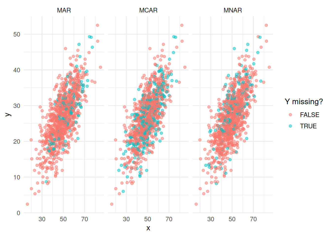
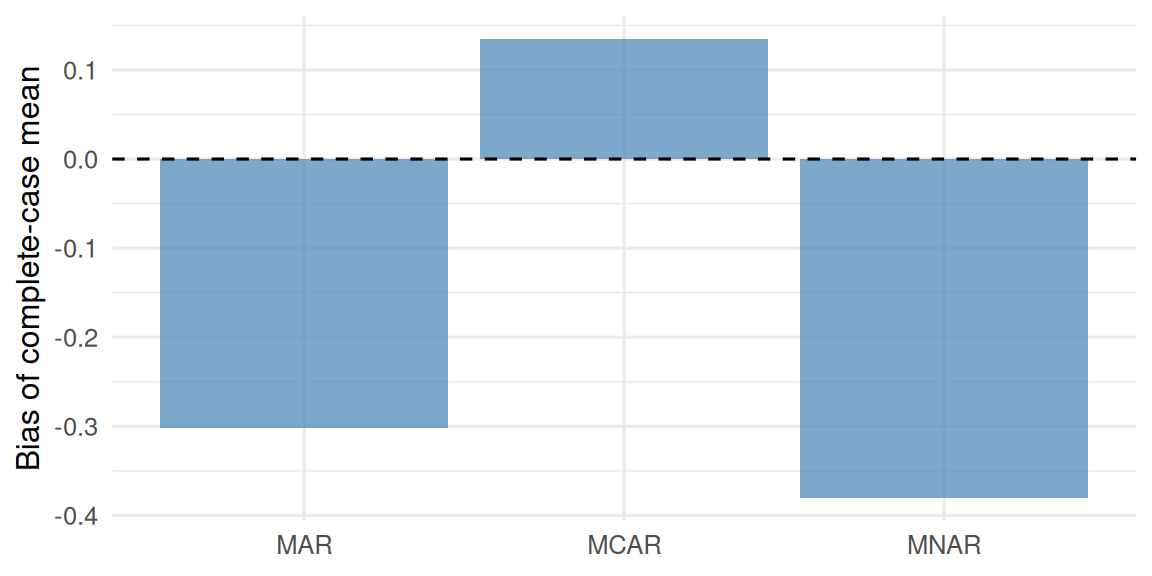
3. Assumptions

Complete-case analysis is the bluntest possible method. It is justified if missingness is MCAR. We will compute the mean of Y on observed rows for each mechanism and compare with the true mean.

4. Conduct

results <- all |>
  group_by(mech) |>
  summarise(
    truth = mean(y),
    cc    = mean(y_obs, na.rm = TRUE),
    bias  = cc - truth,
    pct_missing = mean(is.na(y_obs)) * 100
  )
results
# A tibble: 3 × 5
  mech  truth    cc   bias pct_missing
  <chr> <dbl> <dbl>  <dbl>       <dbl>
1 MAR    26.8  26.5 -0.301        12.7
2 MCAR   26.8  27.0  0.135        28.5
3 MNAR   26.8  26.5 -0.380        14.9
results |>
  ggplot(aes(mech, bias)) +
  geom_col(alpha = 0.7, fill = "steelblue") +
  geom_hline(yintercept = 0, linetype = "dashed") +
  labs(x = NULL, y = "Bias of complete-case mean")

5. Concluding statement

Complete-case estimation of the mean of Y was unbiased under MCAR (bias ≈ 0.13) and meaningfully biased under MAR (-0.3) and MNAR (-0.38), despite the same true mean and similar missingness proportions.

Common pitfalls

  • Using Little’s test as evidence for MCAR.
  • Imputing with a model that omits the analysis outcome.
  • Reporting a sample size inflated by a complete-case filter that hides 40% dropout.
  • Using “the missingness was not significantly related to X” as proof of MAR.

Further reading

  • Little RJA, Rubin DB. Statistical Analysis with Missing Data.
  • van Buuren S (2018), Flexible Imputation of Missing Data.
  • Sterne JA et al. (2009), Multiple imputation for missing data in epidemiological and clinical research.

Session info

sessionInfo()
R version 4.4.1 (2024-06-14)
Platform: x86_64-pc-linux-gnu
Running under: Ubuntu 24.04.4 LTS

Matrix products: default
BLAS:   /usr/lib/x86_64-linux-gnu/openblas-pthread/libblas.so.3 
LAPACK: /usr/lib/x86_64-linux-gnu/openblas-pthread/libopenblasp-r0.3.26.so;  LAPACK version 3.12.0

locale:
 [1] LC_CTYPE=C.UTF-8       LC_NUMERIC=C           LC_TIME=C.UTF-8       
 [4] LC_COLLATE=C.UTF-8     LC_MONETARY=C.UTF-8    LC_MESSAGES=C.UTF-8   
 [7] LC_PAPER=C.UTF-8       LC_NAME=C              LC_ADDRESS=C          
[10] LC_TELEPHONE=C         LC_MEASUREMENT=C.UTF-8 LC_IDENTIFICATION=C   

time zone: UTC
tzcode source: system (glibc)

attached base packages:
[1] stats     graphics  grDevices utils     datasets  methods   base     

other attached packages:
 [1] lubridate_1.9.5 forcats_1.0.1   stringr_1.6.0   dplyr_1.2.1    
 [5] purrr_1.2.2     readr_2.2.0     tidyr_1.3.2     tibble_3.3.1   
 [9] ggplot2_4.0.3   tidyverse_2.0.0

loaded via a namespace (and not attached):
 [1] gtable_0.3.6       jsonlite_2.0.0     compiler_4.4.1     tidyselect_1.2.1  
 [5] scales_1.4.0       yaml_2.3.12        fastmap_1.2.0      R6_2.6.1          
 [9] labeling_0.4.3     generics_0.1.4     knitr_1.51         htmlwidgets_1.6.4 
[13] pillar_1.11.1      RColorBrewer_1.1-3 tzdb_0.5.0         rlang_1.2.0       
[17] utf8_1.2.6         stringi_1.8.7      xfun_0.57          S7_0.2.2          
[21] otel_0.2.0         timechange_0.4.0   cli_3.6.6          withr_3.0.2       
[25] magrittr_2.0.5     digest_0.6.39      grid_4.4.1         hms_1.1.4         
[29] lifecycle_1.0.5    vctrs_0.7.3        evaluate_1.0.5     glue_1.8.1        
[33] farver_2.1.2       rmarkdown_2.31     tools_4.4.1        pkgconfig_2.0.3   
[37] htmltools_0.5.9