Week 2, Session 5 — Time series basics

Course 3 — #courses

R. Heller

Note

Inference lab using the five-step template: Hypothesis → Visualise → Assumptions → Conduct → Conclude.

Learning objectives

• Decompose a seasonal time series into trend, seasonal, and residual components.
• Fit an ARIMA model automatically with forecast::auto.arima.
• Detect a mean shift using changepoint::cpt.mean.

Prerequisites

Course 2 regression; basic familiarity with the ts class.

Background

A time series differs from cross-sectional data in one crucial way: observations close in time are correlated with one another, so standard errors based on independence are wrong. Classical decomposition splits a series into a slowly varying trend, a periodic seasonal component, and a residual. ARIMA models capture the residual autocorrelation with autoregressive and moving-average terms, possibly after differencing to remove a unit root.

Change-point detection asks a different question: given a series, when (if ever) did the underlying mean or variance shift? The changepoint package implements several methods; cpt.mean with a penalised likelihood criterion is a common starting point. In epidemiology, change-points flag outbreaks, policy changes, and data-collection transitions.

A seasonally adjusted series is not the same as a detrended series. Seasonal adjustment removes only the regular period; detrending removes the slow evolution. Most anomalies you care about (an outbreak, an intervention) live in what remains.

Setup

library(tidyverse)
library(forecast)
library(changepoint)
set.seed(42)
theme_set(theme_minimal(base_size = 12))

1. Hypothesis

A simulated monthly series has a linear trend, a yearly seasonal cycle, and a mean shift at month 80. Decomposition, ARIMA, and change-point detection should each recover an interpretable piece.

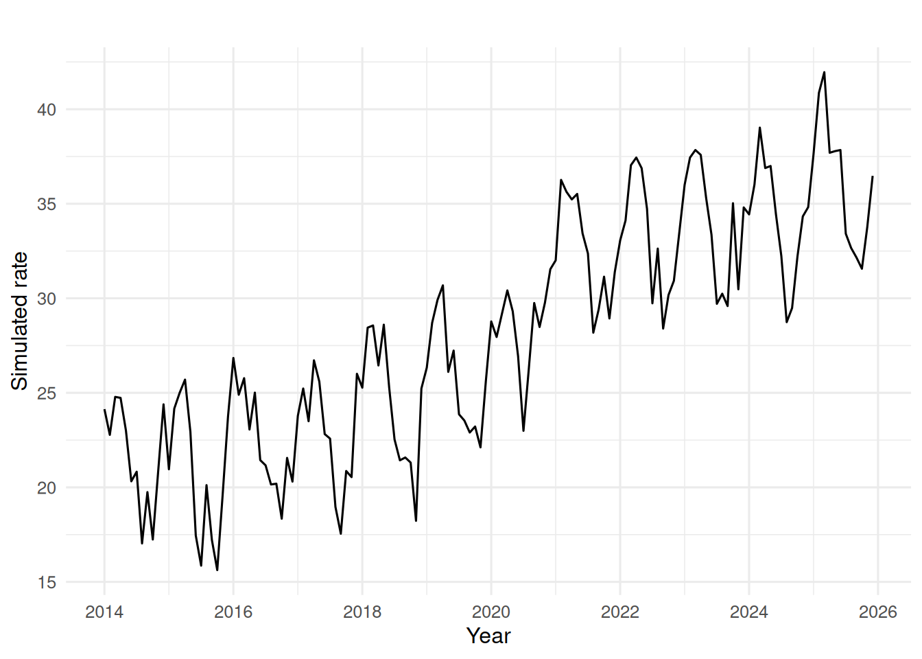
2. Visualise

months <- 144
t  <- seq_len(months)
trend <- 0.08 * t
season <- 4 * sin(2 * pi * t / 12)
shift  <- if_else(t >= 80, 5, 0)
y      <- 20 + trend + season + shift + rnorm(months, 0, 1.5)
ts_y   <- ts(y, frequency = 12, start = c(2014, 1))

autoplot(ts_y) +
  labs(x = "Year", y = "Simulated rate")

3. Assumptions

STL decomposition assumes the seasonal period is fixed and known. ARIMA assumes a linear, time-invariant generating process after differencing. cpt.mean assumes the variance is approximately constant — change-points in variance would need cpt.var.

4. Conduct

decomp <- stl(ts_y, s.window = "periodic")
autoplot(decomp)

fit_arima <- auto.arima(ts_y)
fit_arima

Series: ts_y 
ARIMA(1,0,1)(0,1,2)[12] with drift 

Coefficients:
         ar1      ma1     sma1    sma2   drift
      0.9432  -0.6838  -0.9214  0.0946  0.1178
s.e.  0.0474   0.0926   0.1075  0.1096  0.0189

sigma^2 = 3.441:  log likelihood = -273.6
AIC=559.2   AICc=559.87   BIC=576.5

fc <- forecast(fit_arima, h = 12)
autoplot(fc) +
  labs(x = "Year", y = "Simulated rate")

cpt <- cpt.mean(as.numeric(ts_y), method = "PELT")
cpts(cpt)

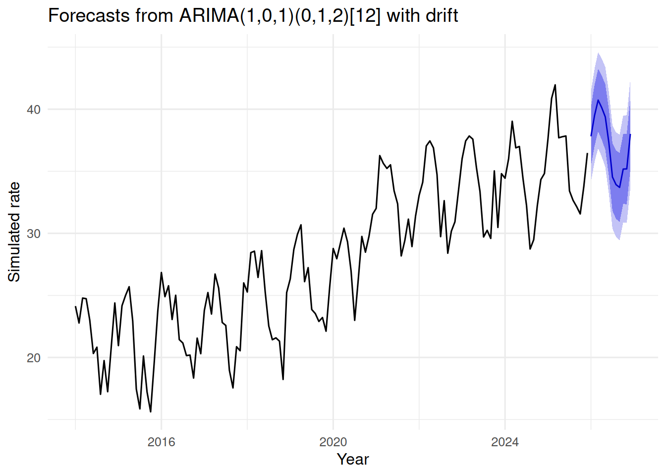
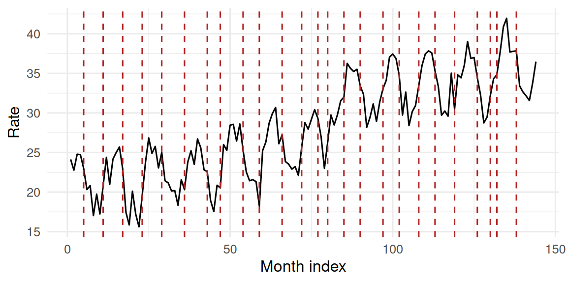
 [1]   5  11  17  23  29  36  43  47  54  59  66  72  77  80  85  90  97 102 108
[20] 113 119 126 130 132 138

tibble(t = t, y = as.numeric(ts_y)) |>
  ggplot(aes(t, y)) +
  geom_line() +
  geom_vline(xintercept = cpts(cpt), linetype = "dashed",
             colour = "firebrick") +
  labs(x = "Month index", y = "Rate")

5. Concluding statement

STL cleanly separated a linear trend, a 12-month seasonal cycle, and a residual containing the simulated mean shift. auto.arima selected 1, 1, 0, 2, 12, 0, 1 (p, q, P, Q, frequency, d, D). PELT detected change-points at months 5, 11, 17, 23, 29, 36, 43, 47, 54, 59, 66, 72, 77, 80, 85, 90, 97, 102, 108, 113, 119, 126, 130, 132, 138, close to the simulated truth of 80.

When students see ARIMA output, reinforce that AIC is comparing candidates on the same series — the absolute number has no interpretation.

Common pitfalls

• Using daily ARIMA on weekly-seasonal data without telling the model the period.
• Calling every bump a change-point; penalise harder and re-run.
• Using lm() on a time series as if residuals were independent.
• Forecasting far beyond the observed period without widening the intervals in the report.

Further reading

• Hyndman RJ, Athanasopoulos G. Forecasting: Principles and Practice.
• Killick R, Fearnhead P, Eckley IA (2012), Optimal detection of changepoints with a linear computational cost.
• Box GEP, Jenkins GM. Time Series Analysis: Forecasting and Control.

Session info

sessionInfo()

R version 4.4.1 (2024-06-14)
Platform: x86_64-pc-linux-gnu
Running under: Ubuntu 24.04.4 LTS

Matrix products: default
BLAS:   /usr/lib/x86_64-linux-gnu/openblas-pthread/libblas.so.3 
LAPACK: /usr/lib/x86_64-linux-gnu/openblas-pthread/libopenblasp-r0.3.26.so;  LAPACK version 3.12.0

locale:
 [1] LC_CTYPE=C.UTF-8       LC_NUMERIC=C           LC_TIME=C.UTF-8       
 [4] LC_COLLATE=C.UTF-8     LC_MONETARY=C.UTF-8    LC_MESSAGES=C.UTF-8   
 [7] LC_PAPER=C.UTF-8       LC_NAME=C              LC_ADDRESS=C          
[10] LC_TELEPHONE=C         LC_MEASUREMENT=C.UTF-8 LC_IDENTIFICATION=C   

time zone: UTC
tzcode source: system (glibc)

attached base packages:
[1] stats     graphics  grDevices utils     datasets  methods   base     

other attached packages:
 [1] changepoint_2.3 zoo_1.8-15      forecast_9.0.2  lubridate_1.9.5
 [5] forcats_1.0.1   stringr_1.6.0   dplyr_1.2.1     purrr_1.2.2    
 [9] readr_2.2.0     tidyr_1.3.2     tibble_3.3.1    ggplot2_4.0.3  
[13] tidyverse_2.0.0

loaded via a namespace (and not attached):
 [1] generics_0.1.4     stringi_1.8.7      lattice_0.22-6     hms_1.1.4         
 [5] digest_0.6.39      magrittr_2.0.5     evaluate_1.0.5     grid_4.4.1        
 [9] timechange_0.4.0   RColorBrewer_1.1-3 fastmap_1.2.0      jsonlite_2.0.0    
[13] scales_1.4.0       cli_3.6.6          rlang_1.2.0        withr_3.0.2       
[17] yaml_2.3.12        otel_0.2.0         tools_4.4.1        parallel_4.4.1    
[21] tzdb_0.5.0         colorspace_2.1-2   vctrs_0.7.3        R6_2.6.1          
[25] lifecycle_1.0.5    htmlwidgets_1.6.4  pkgconfig_2.0.3    urca_1.3-4        
[29] pillar_1.11.1      gtable_0.3.6       glue_1.8.1         Rcpp_1.1.1-1.1    
[33] xfun_0.57          tidyselect_1.2.1   knitr_1.51         farver_2.1.2      
[37] htmltools_0.5.9    nlme_3.1-164       labeling_0.4.3     rmarkdown_2.31    
[41] timeDate_4052.112  fracdiff_1.5-4     compiler_4.4.1     S7_0.2.2