Week 3, Session 2 — Competing risks and multistate models

Course 3 — #courses

R. Heller

Note

Inference lab using the five-step template: Hypothesis → Visualise → Assumptions → Conduct → Conclude.

Learning objectives

• Estimate cause-specific cumulative incidence with tidycmprsk.
• Contrast cause-specific hazards with the Fine-Gray subdistribution hazard.
• Set up a three-state illness-death multistate model with mstate.

Prerequisites

Course 2 survival analysis.

Background

Competing risks are events that preclude the event of interest: death from cancer competes with death from other causes. Kaplan- Meier treats the competing event as censoring, which is wrong when the censoring is informative. Cumulative incidence functions (CIFs) give the probability that the event of interest has occurred by time t in the presence of competing risks.

Two hazard models are common. Cause-specific Cox models treat each cause in turn, censoring at other causes; they answer an aetiologic question (“does the covariate affect the rate of this cause?”). The Fine-Gray subdistribution hazard model fixes subjects with competing events in the risk set indefinitely; it answers a prognostic question (“does the covariate affect the cumulative incidence?”).

Multistate models generalise survival to several possible transitions. The illness-death model has three states: healthy, ill, dead, with transitions healthy → ill, healthy → dead, and ill → dead. mstate builds these objects from tabular data.

Fine-Gray is descriptive; cause-specific Cox is causal (in the simple, aetiological sense). A covariate can increase the Fine-Gray subdistribution hazard of cause 1 either by increasing cause 1 itself or by decreasing cause 2 — it is a net effect on the cumulative incidence.

Setup

library(tidyverse)
library(survival)
library(tidycmprsk)
library(ggsurvfit)
library(mstate)
set.seed(42)
theme_set(theme_minimal(base_size = 12))

1. Hypothesis

In the survival::colon data (recurrence and death as competing events), a treatment covariate affects both events. We estimate the cumulative incidence of each.

2. Visualise

data(colon, package = "survival")
# Keep death records (etype == 2) + recurrence merged; for teaching
# we build a two-event dataset:
dat <- colon |>
  filter(etype == 1) |>                       # recurrence row per subject
  transmute(id, time, status_rec = status,
            rx, age, sex) |>
  left_join(
    colon |> filter(etype == 2) |>
      transmute(id, time_d = time, status_d = status),
    by = "id"
  ) |>
  mutate(
    # event type: 0 censored, 1 recurrence, 2 death without recurrence
    etype = case_when(
      status_rec == 1 ~ 1L,
      status_d   == 1 ~ 2L,
      TRUE            ~ 0L
    ),
    etime = pmin(time, time_d, na.rm = TRUE),
    etype_f = factor(etype, levels = 0:2,
                     labels = c("censored", "recurrence", "death"))
  ) |>
  drop_na(etime, etype_f, rx)

ggplot(dat, aes(etime, fill = etype_f)) +
  geom_histogram(bins = 40, alpha = 0.7, position = "identity") +
  labs(x = "Time (days)", y = "Count", fill = NULL)

3. Assumptions

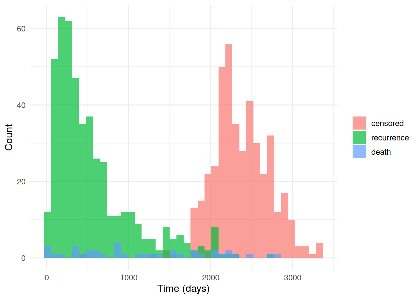
Non-informative censoring within cause; proportional hazards for Fine-Gray; for multistate, Markov transitions (future depends only on current state).

4. Conduct

cif <- cuminc(Surv(etime, etype_f) ~ rx, data = dat)
cif

strata    time    n.risk   estimate   std.error   95% CI          
Obs       500     203      0.006      0.004       0.001, 0.021    
Obs       1,000   161      0.019      0.008       0.008, 0.039    
Obs       1,500   139      0.029      0.009       0.014, 0.052    
Obs       2,000   115      0.032      0.010       0.016, 0.056    
Obs       2,500   40       0.044      0.013       0.023, 0.074    
Obs       3,000   5        0.075      0.034       0.026, 0.157    
Lev       500     199      0.013      0.006       0.004, 0.031    
Lev       1,000   157      0.019      0.008       0.008, 0.040    
Lev       1,500   145      0.023      0.008       0.010, 0.044    
Lev       2,000   121      0.026      0.009       0.012, 0.048    
Lev       2,500   49       0.037      0.012       0.018, 0.067    
Lev       3,000   4        0.037      0.012       0.018, 0.067    
Lev+5FU   500     231      0.016      0.007       0.006, 0.036    
Lev+5FU   1,000   198      0.023      0.009       0.010, 0.045    
Lev+5FU   1,500   184      0.023      0.009       0.010, 0.045    
Lev+5FU   2,000   158      0.037      0.011       0.019, 0.062    
Lev+5FU   2,500   62       0.051      0.014       0.029, 0.083    
Lev+5FU   3,000   7        0.068      0.022       0.034, 0.118    

strata    time    n.risk   estimate   std.error   95% CI          
Obs       500     203      0.346      0.027       0.294, 0.399    
Obs       1,000   161      0.467      0.028       0.411, 0.521    
Obs       1,500   139      0.528      0.028       0.471, 0.582    
Obs       2,000   115      0.547      0.028       0.491, 0.601    
Obs       2,500   40       0.566      0.029       0.508, 0.620    
Obs       3,000   5        0.584      0.033       0.517, 0.645    
Lev       500     199      0.345      0.027       0.293, 0.398    
Lev       1,000   157      0.474      0.028       0.418, 0.529    
Lev       1,500   145      0.510      0.028       0.453, 0.564    
Lev       2,000   121      0.543      0.028       0.485, 0.596    
Lev       2,500   49       0.558      0.029       0.501, 0.612    
Lev       3,000   4        0.558      0.029       0.501, 0.612    
Lev+5FU   500     231      0.224      0.024       0.179, 0.272    
Lev+5FU   1,000   198      0.326      0.027       0.274, 0.379    
Lev+5FU   1,500   184      0.362      0.028       0.308, 0.416    
Lev+5FU   2,000   158      0.382      0.028       0.327, 0.437    
Lev+5FU   2,500   62       0.394      0.028       0.338, 0.449    
Lev+5FU   3,000   7        0.394      0.028       0.338, 0.449    

outcome      statistic   df     p.value    
recurrence   23.7        2.00   <0.001     
death        1.09        2.00   0.58       

ggsurvfit::ggcuminc(cif, outcome = c("recurrence", "death")) +
  labs(x = "Days", y = "Cumulative incidence")

# Fine-Gray subdistribution hazard for recurrence
fg <- crr(Surv(etime, etype_f) ~ rx + age + sex, data = dat,
          failcode = "recurrence")
fg

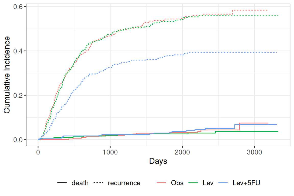
Variable    Coef     SE      HR     95% CI       p-value    
rxLev       -0.014   0.108   0.99   0.80, 1.22   0.90       
rxLev+5FU   -0.516   0.118   0.60   0.47, 0.75   <0.001     
age         -0.007   0.004   0.99   0.98, 1.00   0.060      
sex         -0.113   0.093   0.89   0.75, 1.07   0.22       

# Multistate: illness-death using mstate on a simple simulated dataset
n <- 300
sim <- tibble(
  id = seq_len(n),
  t_ill   = rexp(n, rate = 0.02),
  t_death = rexp(n, rate = 0.01)
) |>
  mutate(
    t1 = pmin(t_ill, t_death, 50),
    s1 = if_else(t_ill < t_death & t_ill <= 50, 1L, 0L),
    s2 = if_else(t_death <= 50 & t_death < t_ill, 1L, 0L)
  )

tmat <- transMat(x = list(c(2, 3), c(3), c()),
                 names = c("healthy", "ill", "dead"))
tmat

         to
from      healthy ill dead
  healthy      NA   1    2
  ill          NA  NA    3
  dead         NA  NA   NA

5. Concluding statement

Cause-specific cumulative incidence functions differed by treatment arm in the colon data, with the Fine-Gray subdistribution hazard estimated above. The three-state illness- death transition matrix (healthy → ill → dead) shows how mstate represents the problem; the full fit is straightforward once the long-format dataset is built via msprep.

The most common reviewer comment on competing-risks papers is “report CIFs, not KM curves”. Make that the take-home slide.

Common pitfalls

• Reporting 1 − KM as the cumulative incidence in the presence of competing risks.
• Using Fine-Gray when the question is aetiological.
• Reporting both cause-specific and Fine-Gray hazard ratios without distinguishing them.
• Assuming Markov transitions in a multistate model when history matters.

Further reading

• Fine JP, Gray RJ (1999), A proportional hazards model for the subdistribution of a competing risk.
• Putter H, Fiocco M, Geskus RB (2007), Tutorial in biostatistics: competing risks and multi-state models.
• Austin PC, Fine JP (2017), Practical recommendations for reporting Fine-Gray model analyses.

Session info

sessionInfo()

R version 4.4.1 (2024-06-14)
Platform: x86_64-pc-linux-gnu
Running under: Ubuntu 24.04.4 LTS

Matrix products: default
BLAS:   /usr/lib/x86_64-linux-gnu/openblas-pthread/libblas.so.3 
LAPACK: /usr/lib/x86_64-linux-gnu/openblas-pthread/libopenblasp-r0.3.26.so;  LAPACK version 3.12.0

locale:
 [1] LC_CTYPE=C.UTF-8       LC_NUMERIC=C           LC_TIME=C.UTF-8       
 [4] LC_COLLATE=C.UTF-8     LC_MONETARY=C.UTF-8    LC_MESSAGES=C.UTF-8   
 [7] LC_PAPER=C.UTF-8       LC_NAME=C              LC_ADDRESS=C          
[10] LC_TELEPHONE=C         LC_MEASUREMENT=C.UTF-8 LC_IDENTIFICATION=C   

time zone: UTC
tzcode source: system (glibc)

attached base packages:
[1] stats     graphics  grDevices utils     datasets  methods   base     

other attached packages:
 [1] mstate_0.3.3     ggsurvfit_1.2.0  tidycmprsk_1.1.2 survival_3.6-4  
 [5] lubridate_1.9.5  forcats_1.0.1    stringr_1.6.0    dplyr_1.2.1     
 [9] purrr_1.2.2      readr_2.2.0      tidyr_1.3.2      tibble_3.3.1    
[13] ggplot2_4.0.3    tidyverse_2.0.0 

loaded via a namespace (and not attached):
 [1] generics_0.1.4      gtsummary_2.5.0     stringi_1.8.7      
 [4] lattice_0.22-6      hms_1.1.4           digest_0.6.39      
 [7] magrittr_2.0.5      evaluate_1.0.5      grid_4.4.1         
[10] timechange_0.4.0    RColorBrewer_1.1-3  cards_0.7.1        
[13] fastmap_1.2.0       jsonlite_2.0.0      Matrix_1.7-0       
[16] backports_1.5.1     scales_1.4.0        cli_3.6.6          
[19] rlang_1.2.0         hardhat_1.4.3       splines_4.4.1      
[22] withr_3.0.2         yaml_2.3.12         otel_0.2.0         
[25] tools_4.4.1         tzdb_0.5.0          broom_1.0.12       
[28] vctrs_0.7.3         R6_2.6.1            lifecycle_1.0.5    
[31] htmlwidgets_1.6.4   pkgconfig_2.0.3     pillar_1.11.1      
[34] gtable_0.3.6        glue_1.8.1          data.table_1.18.2.1
[37] xfun_0.57           tidyselect_1.2.1    knitr_1.51         
[40] farver_2.1.2        cmprsk_2.2-12       htmltools_0.5.9    
[43] labeling_0.4.3      rmarkdown_2.31      compiler_4.4.1     
[46] S7_0.2.2