Week 3, Session 3 — DAGs with dagitty and ggdag
Course 3 — #courses
Note
Workflow lab using the variant template: Goal → Approach → Execution → Check → Report.
Learning objectives
- Express a causal scenario as a directed acyclic graph (DAG).
- Identify confounders, mediators, and colliders from a DAG.
- Use
dagitty::adjustmentSets()to find sufficient adjustment sets.
Prerequisites
Conceptual knowledge of confounding.
Background
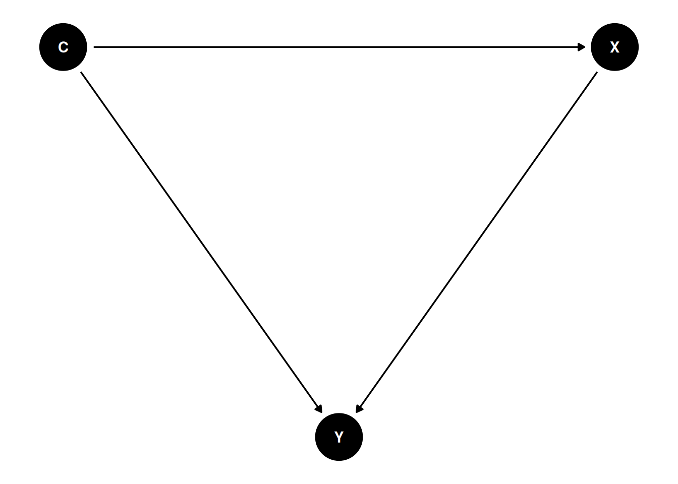
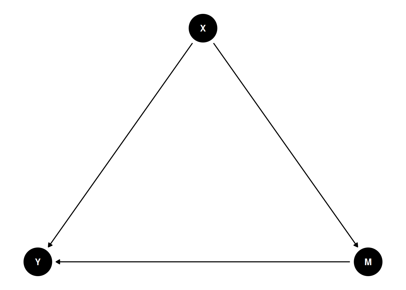
A DAG is a set of variables joined by arrows that encode assumed causal directions. The graph distinguishes three kinds of third variable on a path between exposure and outcome: a confounder is a common cause; a mediator lies on the causal path from exposure to outcome; a collider is a common effect of two variables on the path. The practical upshot is that adjusting for a confounder reduces bias, adjusting for a mediator removes part of the effect you are trying to estimate, and adjusting for a collider creates bias where none existed.
dagitty and ggdag let you declare a DAG in text, visualise it, and then query it for adjustment sets — the minimal variable sets that block all back-door paths from exposure to outcome without opening new ones. The right adjustment set depends on the question. For the total effect of X on Y, you want to close all back-door paths but leave mediators alone; for the direct effect, you also block mediators.
M-bias is the classic example of collider adjustment: conditioning on a variable that is a common effect of an unmeasured cause of X and an unmeasured cause of Y opens a path and biases the estimate. This is why “adjust for everything” is bad advice.
Setup
1. Goal
Write a confounder, mediator, and collider scenario as DAGs; ask dagitty which variables to adjust for.
2. Approach

3. Execution
{}{ M }4. Check
Simulate dag1 and verify that adjusting for C recovers the true effect while failing to adjust biases it.
        x
0.7042359 x
0.3866581 The unadjusted coefficient is inflated; the adjusted one is close to 0.4 as simulated.
5. Report
A directed acyclic graph is a compact, testable statement of causal assumptions. Dagitty identified the confounder C as the required adjustment set in the first DAG; the collider Z in the third DAG is explicitly not in any adjustment set, and conditioning on it would introduce selection bias.
Common pitfalls
- Listing “every variable we measured” as the adjustment set.
- Adjusting for a mediator and calling the result a total effect.
- Using automated variable selection on observational data without a DAG.
- Drawing the DAG after the analysis.
Further reading
- Textor J et al. (2016), Robust causal inference using directed acyclic graphs: the R package ‘dagitty’.
- Hernán MA, Robins JM. Causal Inference: What If.
- Greenland S, Pearl J, Robins JM (1999), Causal diagrams for epidemiologic research.
Session info
R version 4.5.2 (2025-10-31 ucrt)
Platform: x86_64-w64-mingw32/x64
Running under: Windows 11 x64 (build 26200)

Matrix products: default
  LAPACK version 3.12.1

locale:
[1] LC_COLLATE=English_Germany.utf8  LC_CTYPE=English_Germany.utf8
[3] LC_MONETARY=English_Germany.utf8 LC_NUMERIC=C
[5] LC_TIME=English_Germany.utf8

time zone: Europe/Berlin
tzcode source: internal

attached base packages:
[1] stats     graphics  grDevices utils     datasets  methods   base

other attached packages:
 [1] ggdag_0.2.13    dagitty_0.3-4   lubridate_1.9.5 forcats_1.0.1
 [5] stringr_1.6.0   dplyr_1.2.1     purrr_1.2.2     readr_2.2.0
 [9] tidyr_1.3.2     tibble_3.3.1    ggplot2_4.0.3   tidyverse_2.0.0

loaded via a namespace (and not attached):
 [1] viridis_0.6.5      generics_0.1.4     stringi_1.8.7      hms_1.1.4
 [5] digest_0.6.39      magrittr_2.0.4     evaluate_1.0.5     grid_4.5.2
 [9] timechange_0.4.0   RColorBrewer_1.1-3 fastmap_1.2.0      jsonlite_2.0.0
[13] ggrepel_0.9.8      gridExtra_2.3      viridisLite_0.4.3  scales_1.4.0
[17] tweenr_2.0.3       cli_3.6.6          graphlayouts_1.2.3 rlang_1.2.0
[21] polyclip_1.10-7    tidygraph_1.3.1    cachem_1.1.0       withr_3.0.2
[25] yaml_2.3.12        otel_0.2.0         tools_4.5.2        tzdb_0.5.0
[29] memoise_2.0.1      boot_1.3-32        curl_7.1.0         vctrs_0.7.3
[33] R6_2.6.1           lifecycle_1.0.5    V8_8.2.0           htmlwidgets_1.6.4
[37] MASS_7.3-65        ggraph_2.2.2       pkgconfig_2.0.3    pillar_1.11.1
[41] gtable_0.3.6       glue_1.8.1         Rcpp_1.1.1-1.1     ggforce_0.5.0
[45] xfun_0.57          tidyselect_1.2.1   knitr_1.51         farver_2.1.2
[49] htmltools_0.5.9    igraph_2.3.1       labeling_0.4.3     rmarkdown_2.31
[53] compiler_4.5.2     S7_0.2.2