Week 1, Session 1 — Cross-validation, nested CV, bootstrap .632+

Course 4 — #courses

R. Heller

Note

Workflow labs use the variant template: Goal → Approach → Execution → Check → Report.

Learning objectives

• Implement k-fold and repeated k-fold cross-validation from scratch and with a package, and report an honest generalisation error.
• Explain why selecting a model and tuning a hyperparameter on the same fold inflates performance, and use nested CV to fix it.
• Compute a bootstrap .632+ estimate and say when it is preferable to

Prerequisites

Course 1 material on sampling variability; comfort with caret or base-R model fitting.

Background

Every predictive model reports an error on the data it was fit to. That number is almost always optimistic, because the fit has had a chance to memorise noise as well as signal. Cross-validation and the bootstrap are two resampling strategies that simulate the experience of scoring the model on data it has not seen. They are not interchangeable: they make different trade-offs between bias and variance, and they behave differently under high-dimensional settings.

A particular failure mode that recurs in the applied literature is double dipping: using the same held-out fold both to choose a hyperparameter and to report the final error. The fold is then no longer held out, and the reported error slides back toward the training error. Nested cross-validation is the clean solution: the inner loop picks hyperparameters, the outer loop reports error.

The bootstrap gives a different window onto generalisation. The plain bootstrap resamples with replacement; the .632 and .632+ variants weight the in-bag and out-of-bag errors to reduce bias when the learner overfits. In very small samples the .632+ estimator is often the most stable, and it is worth carrying in your toolbox alongside CV.

A practical note: when you write up a modelling study, the generalisation error is the headline number. If you tuned, you must disclose how. If the inner tuning cost was hidden in the outer fold, a careful reader will notice that the reported error is too good and cannot be reproduced. Nested CV is not a cosmetic fix; it is the difference between a number that generalises and a number that does not.

Setup

library(tidyverse)
library(glmnet)
set.seed(42)
theme_set(theme_minimal(base_size = 12))

1. Goal

Estimate the generalisation error of a lasso on a moderate p, small n simulated regression problem, first naively, then with a proper nested cross-validation.

2. Approach

We simulate n = 120 observations with p = 40 features, of which only 5 are true signal. We will (i) fit a single cv.glmnet, (ii) report the CV-minimising error, then (iii) wrap that in an outer 5-fold loop to show that the inner CV error is optimistic.

n <- 120; p <- 40
X <- matrix(rnorm(n * p), n, p)
beta <- c(rep(1.5, 5), rep(0, p - 5))
y <- as.numeric(X %*% beta + rnorm(n, sd = 1.0))

tibble(yhat_naive = as.numeric(X %*% beta), y = y) |>
  ggplot(aes(yhat_naive, y)) +
  geom_point(alpha = 0.6) +
  geom_abline(slope = 1, intercept = 0, colour = "grey50") +
  labs(x = "True linear predictor", y = "Observed y")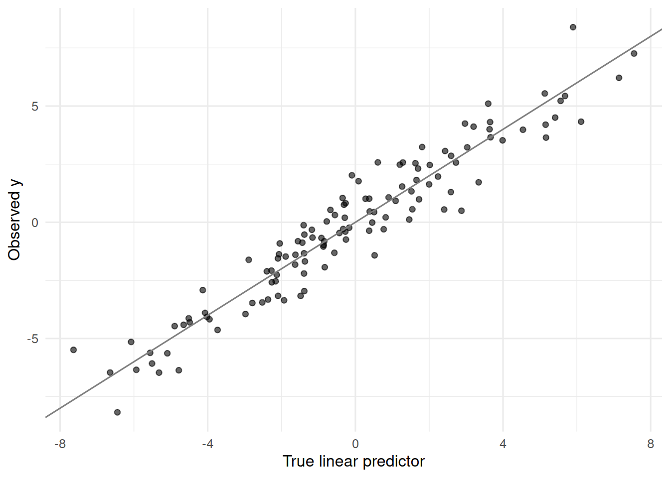

3. Execution

Naive single-layer CV.

cv1 <- cv.glmnet(X, y, alpha = 1, nfolds = 5)
naive_mse <- min(cv1$cvm)
naive_mse

[1] 1.206876

Nested CV. The inner cv.glmnet picks lambda; the outer 5 folds produce the reported MSE.

K <- 5
folds <- sample(rep(1:K, length.out = n))
outer_mse <- numeric(K)
for (k in 1:K) {
  tr <- folds != k; te <- folds == k
  fit_k <- cv.glmnet(X[tr, ], y[tr], alpha = 1, nfolds = 5)
  yhat  <- as.numeric(predict(fit_k, newx = X[te, ], s = "lambda.min"))
  outer_mse[k] <- mean((y[te] - yhat)^2)
}
nested_mse <- mean(outer_mse)
c(naive = naive_mse, nested = nested_mse)

   naive   nested 
1.206876 1.048175 

4. Check

Bootstrap .632+ error as a cross-check.

B <- 50
errs_in <- errs_oob <- numeric(B)
for (b in 1:B) {
  idx <- sample.int(n, n, replace = TRUE)
  oob <- setdiff(seq_len(n), unique(idx))
  fit_b <- cv.glmnet(X[idx, ], y[idx], alpha = 1, nfolds = 5)
  yhat_in  <- as.numeric(predict(fit_b, newx = X[idx, ],  s = "lambda.min"))
  yhat_oob <- as.numeric(predict(fit_b, newx = X[oob, ],  s = "lambda.min"))
  errs_in[b]  <- mean((y[idx] - yhat_in)^2)
  errs_oob[b] <- mean((y[oob] - yhat_oob)^2)
}
err_app <- mean(errs_in); err_oob <- mean(errs_oob)
err_632 <- 0.368 * err_app + 0.632 * err_oob
c(apparent = err_app, oob = err_oob, boot632 = err_632,
  nested = nested_mse)

 apparent       oob   boot632    nested 
0.5199837 1.2632623 0.9897358 1.0481752 

5. Report

On simulated data (n = 120, p = 40, five true signals), a lasso with tuning parameter chosen by 5-fold CV achieved an out-of-sample MSE of 1.05 under nested 5 × 5 CV. The naive single-layer CV understated the error at 1.21; the bootstrap .632 estimator gave 0.99, which bracketed the nested estimate.

The naive number looks tighter, but it reflects the choice of lambda as well as the fit. Only the nested number is a fair estimate of what this procedure — tune-then-fit — will do on new data.

Emphasise that “naive CV” is still useful: it is the inner loop in a nested scheme. The crime is reporting it as the final error.

Common pitfalls

• Tuning on the test fold and reporting the resulting error.
• Using a single 80/20 split in high dimensions; variance across splits can exceed the effect of interest.
• Bootstrapping without tracking in-bag vs out-of-bag, which inflates the estimate back to the apparent error.

Further reading

• Hastie, Tibshirani, Friedman, Elements of Statistical Learning, §7.10–7.11.
• Varma S, Simon R (2006), Bias in error estimation when using cross-validation for model selection.
• Efron B, Tibshirani R (1997), Improvements on cross-validation: the .632+ bootstrap method.

Session info

sessionInfo()

R version 4.4.1 (2024-06-14)
Platform: x86_64-pc-linux-gnu
Running under: Ubuntu 24.04.4 LTS

Matrix products: default
BLAS:   /usr/lib/x86_64-linux-gnu/openblas-pthread/libblas.so.3 
LAPACK: /usr/lib/x86_64-linux-gnu/openblas-pthread/libopenblasp-r0.3.26.so;  LAPACK version 3.12.0

locale:
 [1] LC_CTYPE=C.UTF-8       LC_NUMERIC=C           LC_TIME=C.UTF-8       
 [4] LC_COLLATE=C.UTF-8     LC_MONETARY=C.UTF-8    LC_MESSAGES=C.UTF-8   
 [7] LC_PAPER=C.UTF-8       LC_NAME=C              LC_ADDRESS=C          
[10] LC_TELEPHONE=C         LC_MEASUREMENT=C.UTF-8 LC_IDENTIFICATION=C   

time zone: UTC
tzcode source: system (glibc)

attached base packages:
[1] stats     graphics  grDevices utils     datasets  methods   base     

other attached packages:
 [1] glmnet_5.0      Matrix_1.7-0    lubridate_1.9.5 forcats_1.0.1  
 [5] stringr_1.6.0   dplyr_1.2.1     purrr_1.2.2     readr_2.2.0    
 [9] tidyr_1.3.2     tibble_3.3.1    ggplot2_4.0.3   tidyverse_2.0.0

loaded via a namespace (and not attached):
 [1] generics_0.1.4     shape_1.4.6.1      stringi_1.8.7      lattice_0.22-6    
 [5] hms_1.1.4          digest_0.6.39      magrittr_2.0.5     evaluate_1.0.5    
 [9] grid_4.4.1         timechange_0.4.0   RColorBrewer_1.1-3 iterators_1.0.14  
[13] fastmap_1.2.0      foreach_1.5.2      jsonlite_2.0.0     survival_3.6-4    
[17] scales_1.4.0       codetools_0.2-20   cli_3.6.6          rlang_1.2.0       
[21] splines_4.4.1      withr_3.0.2        yaml_2.3.12        otel_0.2.0        
[25] tools_4.4.1        tzdb_0.5.0         vctrs_0.7.3        R6_2.6.1          
[29] lifecycle_1.0.5    htmlwidgets_1.6.4  pkgconfig_2.0.3    pillar_1.11.1     
[33] gtable_0.3.6       glue_1.8.1         Rcpp_1.1.1-1.1     xfun_0.57         
[37] tidyselect_1.2.1   knitr_1.51         farver_2.1.2       htmltools_0.5.9   
[41] rmarkdown_2.31     labeling_0.4.3     compiler_4.4.1     S7_0.2.2