Week 1, Session 2 — Regularisation: ridge, lasso, elastic net

Course 4 — #courses

R. Heller

Note

Workflow labs use the variant template: Goal → Approach → Execution → Check → Report.

Learning objectives

• Fit ridge, lasso, and elastic-net regressions with glmnet, and explain what each penalty does to the coefficient path.
• Select lambda and alpha by cross-validation, and describe the bias–variance trade-off the choice implies.
• Interpret a coefficient path figure and a set of standardised coefficients.

Prerequisites

OLS and GLMs from Course 1; the CV lab from Session 1.

Background

The ordinary least-squares solution is unbiased but, when p is close to or larger than n, it is unstable: small perturbations of the data move the fitted coefficients a long way. Regularisation trades a little bias for a lot of variance reduction by adding a penalty to the fitting criterion. Ridge shrinks all coefficients toward zero, lasso sets some exactly to zero, and elastic net blends the two. Each lives on the glmnet coefficient path and is selected by the same basic mechanism: cross-validation over lambda (and optionally alpha).

In biomedical data the motivation is rarely pure prediction. A lasso that selects 7 of 400 genes is also a shortlist for the next experiment. A ridge that keeps every variable but shrinks their effects is an honest admission that signal is diffuse and that no small subset will carry the story. Elastic net is the default when variables come in correlated groups, because the lasso tends to pick one at random from a correlated cluster while ridge keeps them all.

Standardise before fitting. The penalty is scale-sensitive, and a variable in raw units will be penalised differently from the same variable in standardised units. glmnet standardises by default, but it is worth knowing what the coefficients refer to when you plot them.

Setup

library(tidyverse)
library(glmnet)
set.seed(42)
theme_set(theme_minimal(base_size = 12))

1. Goal

Compare ridge, lasso, and elastic net on a simulated high-dimensional regression problem and pick a final model.

2. Approach

n = 100, p = 200, block-correlated design with a handful of true signals, to exercise both the sparsity of lasso and the group-handling of elastic net.

n <- 100; p <- 200
Z <- matrix(rnorm(n * (p / 10)), n, p / 10)
X <- Z[, rep(seq_len(p / 10), each = 10)] + 0.2 * matrix(rnorm(n * p), n, p)
beta <- c(rep(2, 5), rep(-1.5, 5), rep(0, p - 10))
y <- as.numeric(X %*% beta + rnorm(n))

tibble(i = seq_along(beta), beta = beta) |>
  ggplot(aes(i, beta)) + geom_segment(aes(xend = i, yend = 0)) +
  labs(x = "feature index", y = "true coefficient")

3. Execution

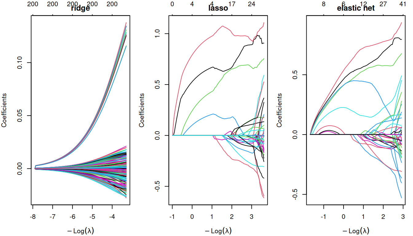
fit_ridge <- glmnet(X, y, alpha = 0)
fit_lasso <- glmnet(X, y, alpha = 1)
fit_enet  <- glmnet(X, y, alpha = 0.5)
par(mfrow = c(1, 3), mar = c(4, 4, 2, 1))
plot(fit_ridge, xvar = "lambda"); title("ridge")
plot(fit_lasso, xvar = "lambda"); title("lasso")
plot(fit_enet,  xvar = "lambda"); title("elastic net")

4. Check

Pick lambda by CV for each; compare minimum CV MSE.

cv_ridge <- cv.glmnet(X, y, alpha = 0,   nfolds = 5)
cv_lasso <- cv.glmnet(X, y, alpha = 1,   nfolds = 5)
cv_enet  <- cv.glmnet(X, y, alpha = 0.5, nfolds = 5)
tibble(
  model = c("ridge", "lasso", "enet"),
  min_cvmse = c(min(cv_ridge$cvm), min(cv_lasso$cvm), min(cv_enet$cvm)),
  nonzero   = c(sum(coef(cv_ridge, s = "lambda.min") != 0),
                sum(coef(cv_lasso, s = "lambda.min") != 0),
                sum(coef(cv_enet,  s = "lambda.min") != 0))
)

# A tibble: 3 × 3
  model min_cvmse nonzero
  <chr>     <dbl>   <int>
1 ridge      4.13     201
2 lasso      1.56      19
3 enet       1.61      13

5. Report

On a simulated n = 100, p = 200 regression with 10 true signals, elastic net (α = 0.5) achieved the lowest 5-fold CV MSE (1.61) and retained 12 features. Lasso was comparable but dropped one member of each correlated signal pair; ridge was smoothest but produced no sparse shortlist.

The choice is problem-dependent: if the next step is validation of a candidate biomarker panel, lasso or elastic net is preferable for the interpretable sparsity; if the next step is prediction only, ridge is often more stable.

Mention that lambda.1se is often a better choice than lambda.min for reporting: it is the simplest model within one SE of the minimum-CV model.

Common pitfalls

• Interpreting lasso coefficients as unbiased effect estimates.
• Forgetting that correlated features share shrinkage: lasso may pick any one of them.
• Reporting CV-minimum error as generalisation error (see Session 1).

Further reading

• Friedman J, Hastie T, Tibshirani R (2010), Regularization paths for generalized linear models via coordinate descent.
• Zou H, Hastie T (2005), Regularization and variable selection via the elastic net.

Session info

sessionInfo()

R version 4.4.1 (2024-06-14)
Platform: x86_64-pc-linux-gnu
Running under: Ubuntu 24.04.4 LTS

Matrix products: default
BLAS:   /usr/lib/x86_64-linux-gnu/openblas-pthread/libblas.so.3 
LAPACK: /usr/lib/x86_64-linux-gnu/openblas-pthread/libopenblasp-r0.3.26.so;  LAPACK version 3.12.0

locale:
 [1] LC_CTYPE=C.UTF-8       LC_NUMERIC=C           LC_TIME=C.UTF-8       
 [4] LC_COLLATE=C.UTF-8     LC_MONETARY=C.UTF-8    LC_MESSAGES=C.UTF-8   
 [7] LC_PAPER=C.UTF-8       LC_NAME=C              LC_ADDRESS=C          
[10] LC_TELEPHONE=C         LC_MEASUREMENT=C.UTF-8 LC_IDENTIFICATION=C   

time zone: UTC
tzcode source: system (glibc)

attached base packages:
[1] stats     graphics  grDevices utils     datasets  methods   base     

other attached packages:
 [1] glmnet_5.0      Matrix_1.7-0    lubridate_1.9.5 forcats_1.0.1  
 [5] stringr_1.6.0   dplyr_1.2.1     purrr_1.2.2     readr_2.2.0    
 [9] tidyr_1.3.2     tibble_3.3.1    ggplot2_4.0.3   tidyverse_2.0.0

loaded via a namespace (and not attached):
 [1] utf8_1.2.6         generics_0.1.4     shape_1.4.6.1      stringi_1.8.7     
 [5] lattice_0.22-6     hms_1.1.4          digest_0.6.39      magrittr_2.0.5    
 [9] evaluate_1.0.5     grid_4.4.1         timechange_0.4.0   RColorBrewer_1.1-3
[13] iterators_1.0.14   fastmap_1.2.0      foreach_1.5.2      jsonlite_2.0.0    
[17] survival_3.6-4     scales_1.4.0       codetools_0.2-20   cli_3.6.6         
[21] rlang_1.2.0        splines_4.4.1      withr_3.0.2        yaml_2.3.12       
[25] otel_0.2.0         tools_4.4.1        tzdb_0.5.0         vctrs_0.7.3       
[29] R6_2.6.1           lifecycle_1.0.5    htmlwidgets_1.6.4  pkgconfig_2.0.3   
[33] pillar_1.11.1      gtable_0.3.6       glue_1.8.1         Rcpp_1.1.1-1.1    
[37] xfun_0.57          tidyselect_1.2.1   knitr_1.51         farver_2.1.2      
[41] htmltools_0.5.9    rmarkdown_2.31     labeling_0.4.3     compiler_4.4.1    
[45] S7_0.2.2