Week 1, Session 4 — Clustering: k-means, hierarchical, model-based

Course 4 — #courses

R. Heller

Note

Workflow labs use the variant template: Goal → Approach → Execution → Check → Report.

Learning objectives

• Fit k-means and hierarchical clusterings, and choose k by elbow and silhouette.
• Fit a model-based clustering with mclust and select the number of components by BIC.
• Explain why “number of clusters” is often not the right question.

Prerequisites

PCA from Session 3; distance and linkage from Course 1.

Background

Clustering is a search for structure in unlabelled data, and unlike classification it has no gold standard. Any algorithm will return a partition if asked to, and the partitions it returns depend on assumptions about what a cluster is. K-means assumes roughly spherical, equal-variance clusters and needs k in advance. Hierarchical clustering produces a nested sequence of partitions at every k, which you cut at a level you choose. Model-based clustering fits a Gaussian mixture and selects k by information criterion, which at least makes the assumption explicit.

In biomedicine, the honest version of “how many clusters?” is usually “is there more than one?” A good clustering lab focuses on stability and interpretability of the partition rather than on the number returned.

When you report a clustering, report the number of clusters, the criterion used to select it, a visualisation in a 2-D projection (PCA or UMAP), and the size and key features of each cluster. Do not report p-values for cluster labels against the data that produced the labels; that circularity is a classic error.

Setup

library(tidyverse)
library(mclust)
library(cluster)
set.seed(42)
theme_set(theme_minimal(base_size = 12))

1. Goal

Cluster a simulated dataset with three known groups using three algorithms, and see which recovers the structure.

2. Approach

Three Gaussian blobs in 5 dimensions with different sizes.

make_blob <- function(n, mu, sd = 1) matrix(rnorm(n * 5, 0, sd), n, 5) +
  rep(mu, each = n)
X <- rbind(
  make_blob(60, c(0, 0, 0, 0, 0)),
  make_blob(40, c(3, 0, 0, 0, 0)),
  make_blob(30, c(0, 3, 0, 0, 0))
)
true_lbl <- rep(c("A", "B", "C"), c(60, 40, 30))

pc <- prcomp(X)$x[, 1:2]
tibble(PC1 = pc[, 1], PC2 = pc[, 2], group = true_lbl) |>
  ggplot(aes(PC1, PC2, colour = group)) + geom_point(alpha = 0.7)

3. Execution

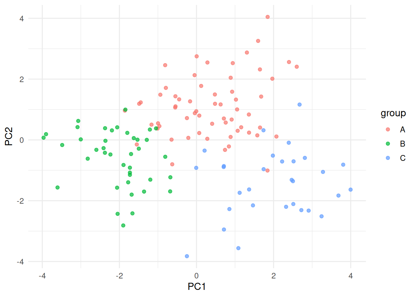
K-means with k sweep; silhouette.

wss <- sapply(2:8, function(k) kmeans(X, centers = k, nstart = 10)$tot.withinss)
sil <- sapply(2:8, function(k) {
  km <- kmeans(X, centers = k, nstart = 10)
  mean(silhouette(km$cluster, dist(X))[, 3])
})
tibble(k = 2:8, wss = wss, sil = sil) |>
  pivot_longer(-k) |>
  ggplot(aes(k, value)) + geom_line() + geom_point() +
  facet_wrap(~ name, scales = "free_y")

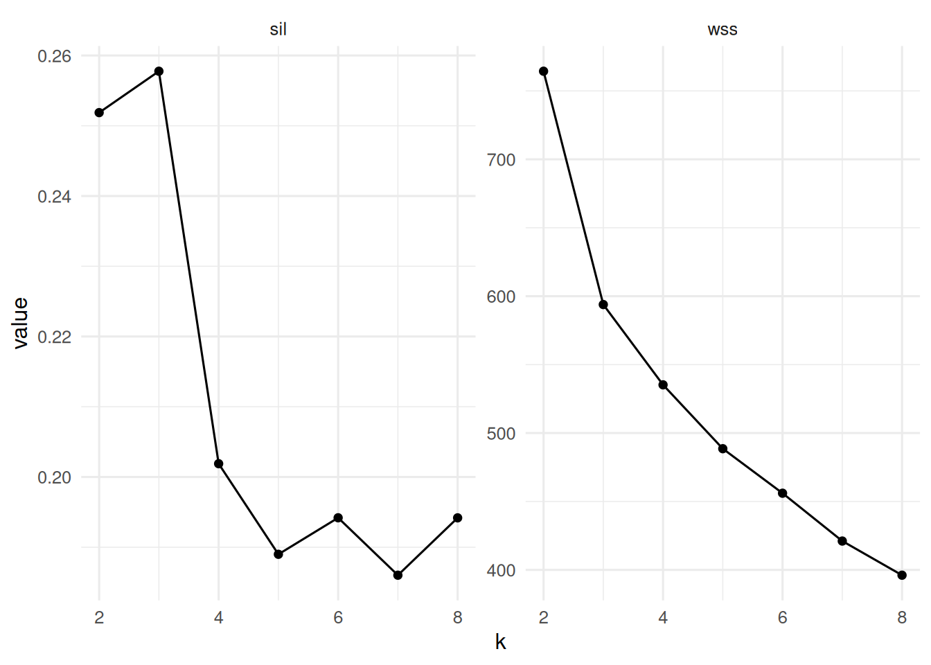
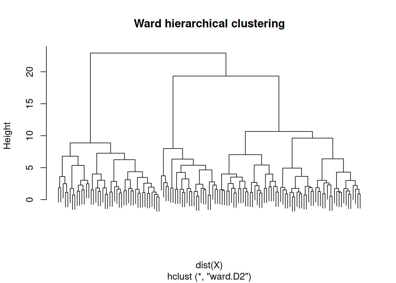
Hierarchical with Ward linkage.

hc <- hclust(dist(X), method = "ward.D2")
plot(hc, labels = FALSE, main = "Ward hierarchical clustering")

4. Check

Model-based clustering by BIC.

mc <- Mclust(X, G = 1:6)
summary(mc)

---------------------------------------------------- 
Gaussian finite mixture model fitted by EM algorithm 
---------------------------------------------------- 

Mclust EII (spherical, equal volume) model with 3 components: 

 log-likelihood   n df       BIC      ICL
      -1018.943 130 18 -2125.503 -2151.66

Clustering table:
 1  2  3 
51 53 26 

5. Report

On three simulated Gaussian blobs (n = 130 in R⁵), model-based clustering selected G = 3 by BIC; k-means with k = 3 maximised mean silhouette (0.26). Hierarchical clustering with Ward linkage produced a dendrogram consistent with three primary branches.

When the generating model is actually Gaussian, mclust tends to win. On real data, no single method is best; the test is whether the partition is stable under resampling and interpretable in terms of the features.

Show how to bootstrap the clustering and compute an ARI across resamples to quantify stability if time.

Common pitfalls

• Treating k-means output as ground truth; it is an optimisation answer given k.
• Running hierarchical clustering on a very large dataset without noting the O(n²) memory cost.
• Testing post-hoc differences between clusters with the same data that produced them.

Further reading

• Fraley C, Raftery AE (2002), Model-based clustering, discriminant analysis, and density estimation.
• Hastie, Tibshirani, Friedman, ESL, §14.3.

Session info

sessionInfo()

R version 4.4.1 (2024-06-14)
Platform: x86_64-pc-linux-gnu
Running under: Ubuntu 24.04.4 LTS

Matrix products: default
BLAS:   /usr/lib/x86_64-linux-gnu/openblas-pthread/libblas.so.3 
LAPACK: /usr/lib/x86_64-linux-gnu/openblas-pthread/libopenblasp-r0.3.26.so;  LAPACK version 3.12.0

locale:
 [1] LC_CTYPE=C.UTF-8       LC_NUMERIC=C           LC_TIME=C.UTF-8       
 [4] LC_COLLATE=C.UTF-8     LC_MONETARY=C.UTF-8    LC_MESSAGES=C.UTF-8   
 [7] LC_PAPER=C.UTF-8       LC_NAME=C              LC_ADDRESS=C          
[10] LC_TELEPHONE=C         LC_MEASUREMENT=C.UTF-8 LC_IDENTIFICATION=C   

time zone: UTC
tzcode source: system (glibc)

attached base packages:
[1] stats     graphics  grDevices utils     datasets  methods   base     

other attached packages:
 [1] cluster_2.1.8.2 mclust_6.1.2    lubridate_1.9.5 forcats_1.0.1  
 [5] stringr_1.6.0   dplyr_1.2.1     purrr_1.2.2     readr_2.2.0    
 [9] tidyr_1.3.2     tibble_3.3.1    ggplot2_4.0.3   tidyverse_2.0.0

loaded via a namespace (and not attached):
 [1] gtable_0.3.6       jsonlite_2.0.0     compiler_4.4.1     tidyselect_1.2.1  
 [5] scales_1.4.0       yaml_2.3.12        fastmap_1.2.0      R6_2.6.1          
 [9] labeling_0.4.3     generics_0.1.4     knitr_1.51         htmlwidgets_1.6.4 
[13] pillar_1.11.1      RColorBrewer_1.1-3 tzdb_0.5.0         rlang_1.2.0       
[17] stringi_1.8.7      xfun_0.57          S7_0.2.2           otel_0.2.0        
[21] timechange_0.4.0   cli_3.6.6          withr_3.0.2        magrittr_2.0.5    
[25] digest_0.6.39      grid_4.4.1         hms_1.1.4          lifecycle_1.0.5   
[29] vctrs_0.7.3        evaluate_1.0.5     glue_1.8.1         farver_2.1.2      
[33] rmarkdown_2.31     tools_4.4.1        pkgconfig_2.0.3    htmltools_0.5.9