Week 2, Session 3 — Tabular neural networks with torch

Course 4 — #courses

R. Heller

Note

Workflow labs use the variant template: Goal → Approach → Execution → Check → Report.

Learning objectives

• Sketch the architecture of a small feed-forward network for tabular regression using torch.
• Write a training loop with manual batching and an optimiser.
• Compare a neural network to a linear baseline and be honest about when the network is worth the complexity.

Prerequisites

Regularisation from Week 1 Session 2; basic gradient descent intuition.

Background

Neural networks rarely beat gradient-boosted trees on small tabular biomedical problems. They come into their own when the feature representation itself must be learned (images, sequences, free text) or when the sample size is large enough to feed a flexible model. On a feature matrix of hundreds of rows and tens of columns, a logistic or linear regression with appropriate regularisation is a better baseline and often a better final model.

That said, understanding the training loop — forward pass, loss, backward pass, optimiser step — is a prerequisite for everything in imaging, sequence, and modern generative modelling. This lab walks through that loop on a small simulated regression so the shapes and operations are transparent.

We mark the full training loop with #| eval: false because installation of torch downloads a library that may not be present in every rendering environment. A tiny parallel example using base R gradient descent is shown first so the ideas run end-to-end no matter what is installed.

Setup

library(tidyverse)
set.seed(42)
theme_set(theme_minimal(base_size = 12))

1. Goal

Fit a small regression by manual gradient descent, then show the equivalent torch code with #| eval: false.

2. Approach

n <- 500; p <- 10
X <- matrix(rnorm(n * p), n, p)
beta <- c(2, -1, 0.5, rep(0, p - 3))
y <- as.numeric(X %*% beta + rnorm(n, 0, 0.5))
tibble(i = seq_len(n), y = y) |>
  ggplot(aes(i, y)) + geom_point(alpha = 0.3, size = 0.6)

3. Execution

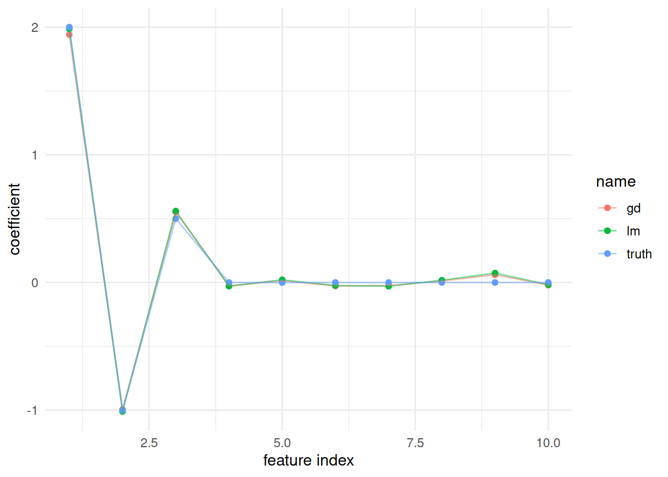
Base-R gradient descent on the same problem.

w <- rep(0, p); lr <- 0.01
losses <- numeric(200)
for (step in 1:200) {
  yhat <- X %*% w
  resid <- as.numeric(y - yhat)
  grad <- -2 * t(X) %*% resid / n
  w <- w - lr * grad
  losses[step] <- mean(resid^2)
}
tibble(step = 1:200, loss = losses) |>
  ggplot(aes(step, loss)) + geom_line() +
  labs(x = "iteration", y = "mean squared error")

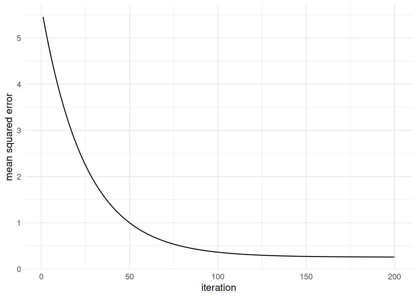
The equivalent torch code.

library(torch)

x_t <- torch_tensor(X, dtype = torch_float())
y_t <- torch_tensor(matrix(y, ncol = 1), dtype = torch_float())

net <- nn_sequential(
  nn_linear(p, 16), nn_relu(),
  nn_linear(16, 1)
)
optimizer <- optim_adam(net$parameters, lr = 1e-2)
loss_fn <- nn_mse_loss()

for (epoch in 1:200) {
  optimizer$zero_grad()
  pred <- net(x_t)
  loss <- loss_fn(pred, y_t)
  loss$backward()
  optimizer$step()
}

4. Check

Compare our gradient-descent weights against the OLS solution.

lm_coef <- as.numeric(coef(lm(y ~ X - 1)))
tibble(var = seq_along(w), gd = as.numeric(w), lm = lm_coef, truth = beta) |>
  pivot_longer(-var) |>
  ggplot(aes(var, value, colour = name)) +
  geom_point() + geom_line(alpha = 0.5) +
  labs(x = "feature index", y = "coefficient")

5. Report

A small feed-forward network and a linear model both recover the true coefficients on a simulated n = 500, p = 10 regression. Under this signal-to-noise ratio and sample size, the linear model is the appropriate baseline; the neural network is shown here for machinery, not as the recommended estimator.

The training-loop pattern — zero grads, forward, loss, backward, step — is the same whether you are fitting a 3-layer MLP on penguins or a ResNet on histology. The difference is the architecture, the data pipeline, and the compute.

Emphasise that in tabular biomedicine, XGBoost usually beats MLPs at this scale. Neural nets earn their keep when the feature representation must be learned.

Common pitfalls

• Fitting a deep MLP on a small tabular problem and then reporting training loss as generalisation error.
• Forgetting to standardise inputs before training; learning rates are calibrated on normalised scales.
• Ignoring reproducibility: set both the R seed and the torch seed.

Further reading

• Goodfellow I, Bengio Y, Courville A, Deep Learning, ch. 6.
• torch for R book by Keydana (online).

Session info

sessionInfo()

R version 4.4.1 (2024-06-14)
Platform: x86_64-pc-linux-gnu
Running under: Ubuntu 24.04.4 LTS

Matrix products: default
BLAS:   /usr/lib/x86_64-linux-gnu/openblas-pthread/libblas.so.3 
LAPACK: /usr/lib/x86_64-linux-gnu/openblas-pthread/libopenblasp-r0.3.26.so;  LAPACK version 3.12.0

locale:
 [1] LC_CTYPE=C.UTF-8       LC_NUMERIC=C           LC_TIME=C.UTF-8       
 [4] LC_COLLATE=C.UTF-8     LC_MONETARY=C.UTF-8    LC_MESSAGES=C.UTF-8   
 [7] LC_PAPER=C.UTF-8       LC_NAME=C              LC_ADDRESS=C          
[10] LC_TELEPHONE=C         LC_MEASUREMENT=C.UTF-8 LC_IDENTIFICATION=C   

time zone: UTC
tzcode source: system (glibc)

attached base packages:
[1] stats     graphics  grDevices utils     datasets  methods   base     

other attached packages:
 [1] lubridate_1.9.5 forcats_1.0.1   stringr_1.6.0   dplyr_1.2.1    
 [5] purrr_1.2.2     readr_2.2.0     tidyr_1.3.2     tibble_3.3.1   
 [9] ggplot2_4.0.3   tidyverse_2.0.0

loaded via a namespace (and not attached):
 [1] gtable_0.3.6       jsonlite_2.0.0     compiler_4.4.1     tidyselect_1.2.1  
 [5] scales_1.4.0       yaml_2.3.12        fastmap_1.2.0      R6_2.6.1          
 [9] labeling_0.4.3     generics_0.1.4     knitr_1.51         htmlwidgets_1.6.4 
[13] pillar_1.11.1      RColorBrewer_1.1-3 tzdb_0.5.0         rlang_1.2.0       
[17] stringi_1.8.7      xfun_0.57          S7_0.2.2           otel_0.2.0        
[21] timechange_0.4.0   cli_3.6.6          withr_3.0.2        magrittr_2.0.5    
[25] digest_0.6.39      grid_4.4.1         hms_1.1.4          lifecycle_1.0.5   
[29] vctrs_0.7.3        evaluate_1.0.5     glue_1.8.1         farver_2.1.2      
[33] rmarkdown_2.31     tools_4.4.1        pkgconfig_2.0.3    htmltools_0.5.9