library(tidyverse)
set.seed(42)
theme_set(theme_minimal(base_size = 12))Week 2, Session 4 — Imaging and sequence models intro
Course 4 — #courses
Note
Workflow labs use the variant template: Goal → Approach → Execution → Check → Report.
Learning objectives
- Describe how a 2-D convolution extracts spatial features from an image.
- Describe how a 1-D convolution or a recurrent layer processes a sequence.
- Recognise when to use a CNN, RNN, or transformer for biomedical data.
Prerequisites
The training loop from Session 3.
Background
Convolutional neural networks (CNNs) exploit the spatial locality of image data: a small filter is slid across the image, producing a feature map for each filter. Stacking convolutional layers lets the network learn increasingly abstract features, from edges to textures to whole tissue structures. In biomedical imaging — histopathology, radiology, dermatology — CNNs underpin the majority of deep-learning applications.
For sequence data — gene sequences, electronic health record time series, wearable signals — the relevant operations are 1-D convolutions and attention. Transformers have become the dominant architecture for long sequences, but 1-D CNNs and gated recurrent networks remain competitive on shorter inputs and are easier to train. This lab illustrates the shape of the computation with a tiny hand-built 2-D convolution and a tiny 1-D convolution; the real training happens with frameworks that we mark #| eval: false.
The conceptual point: image and sequence models share the training loop of Session 3. What differs is the architecture, the data pipeline, and the inductive biases (locality for CNNs, ordered context for RNNs and attention).
Setup
1. Goal
Show manually computed convolutions on a small image and sequence, then sketch the torch code that would perform the same operations inside a trained model.
2. Approach
Create a toy 16×16 image with a bright square.
img <- matrix(0, 16, 16)
img[5:10, 5:10] <- 1
img <- img + matrix(rnorm(256, 0, 0.1), 16, 16)

image(t(img[16:1, ]), col = grey.colors(100), main = "toy image")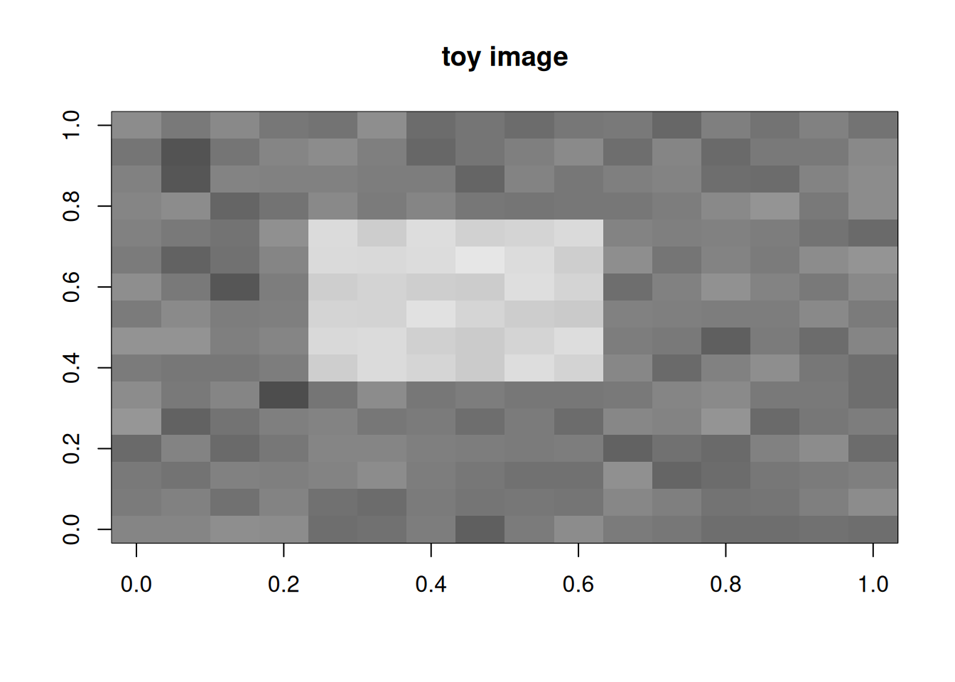
3. Execution
A manual 3×3 edge filter convolved with the image.
kernel <- matrix(c(-1, -1, -1, -1, 8, -1, -1, -1, -1), 3, 3)
conv2d <- function(img, k) {
  kh <- nrow(k); kw <- ncol(k)
  out <- matrix(0, nrow(img) - kh + 1, ncol(img) - kw + 1)
  for (i in seq_len(nrow(out))) for (j in seq_len(ncol(out)))
    out[i, j] <- sum(img[i:(i + kh - 1), j:(j + kw - 1)] * k)
  out
}
feat <- conv2d(img, kernel)
image(t(feat[nrow(feat):1, ]), col = grey.colors(100),
      main = "edge-filter feature map")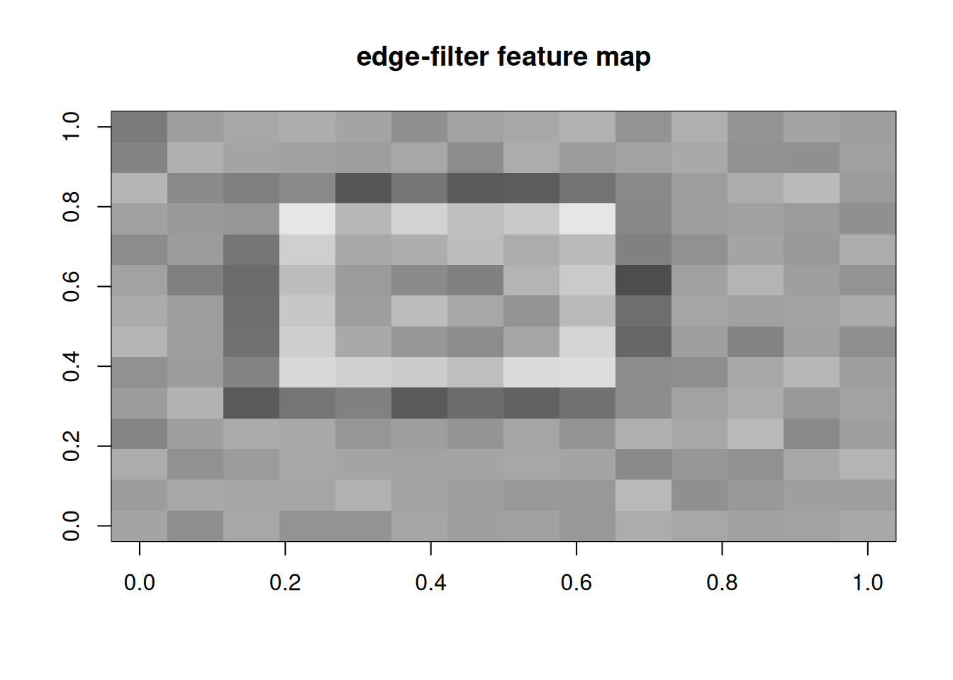
A 1-D convolution on a toy sequence.
seq1 <- c(rep(0, 10), rep(1, 5), rep(0, 10))
conv1d <- function(x, k) {
  out <- numeric(length(x) - length(k) + 1)
  for (i in seq_along(out)) out[i] <- sum(x[i:(i + length(k) - 1)] * k)
  out
}
feat1d <- conv1d(seq1, c(-1, 1))
tibble(i = seq_along(feat1d), v = feat1d) |>
  ggplot(aes(i, v)) + geom_line() +
  labs(x = "position", y = "edge response")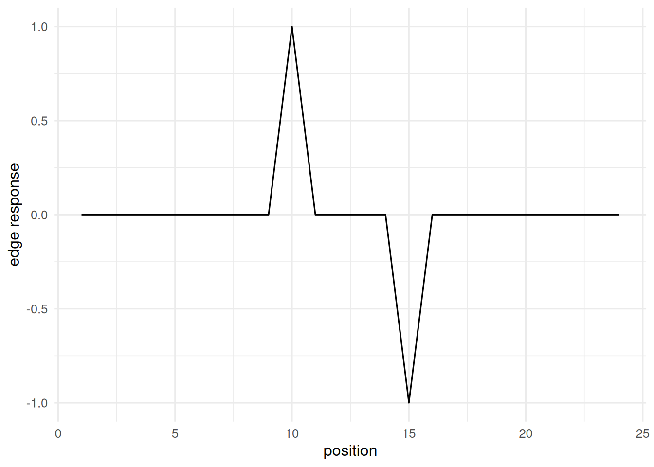
A tiny CNN in torch (sketch only).
library(torch)
cnn <- nn_sequential(
  nn_conv2d(1, 8, kernel_size = 3, padding = 1),
  nn_relu(),
  nn_max_pool2d(2),
  nn_conv2d(8, 16, kernel_size = 3, padding = 1),
  nn_relu(),
  nn_max_pool2d(2),
  nn_flatten(),
  nn_linear(16 * 4 * 4, 10)
)
A 1-D convolutional sequence model sketch.
library(torch)
seq_model <- nn_sequential(
  nn_conv1d(1, 8, kernel_size = 5, padding = 2),
  nn_relu(),
  nn_adaptive_avg_pool1d(1),
  nn_flatten(),
  nn_linear(8, 1)
)
4. Check
Inspect the convolution output shape and magnitude.
dim(feat)[1] 14 14summary(as.numeric(feat)) Min. 1st Qu. Median Mean 3rd Qu. Max.
-3.72594 -0.89661 -0.03791 -0.02161 0.60130 5.48749 5. Report
A 3×3 edge filter applied to a 16×16 toy image produced a feature map of shape 14×14, with responses concentrated at the boundary of the bright square. Analogous 1-D convolutions applied to a binary step sequence produce sharp derivative-like responses at the transitions.
Real CNNs and sequence models compose many such filters, learned from data. The lab establishes the building block so the architectures in the literature read as stacks of familiar operations, not black boxes.
If time, show that a random filter gives noise; the task of training is to learn filters that respond to salient features.
Common pitfalls
- Applying a CNN to tabular data; locality inductive bias is wasted.
- Forgetting input channel and batch dimensions in
torch. - Comparing accuracy of sequence models without specifying the tokenisation used.
Further reading
- LeCun Y, Bengio Y, Hinton G (2015), Deep learning.
- Vaswani A et al. (2017), Attention is all you need.
Session info
sessionInfo()R version 4.5.2 (2025-10-31 ucrt)
Platform: x86_64-w64-mingw32/x64
Running under: Windows 11 x64 (build 26200)
Matrix products: default
LAPACK version 3.12.1
locale:
[1] LC_COLLATE=English_Germany.utf8 LC_CTYPE=English_Germany.utf8
[3] LC_MONETARY=English_Germany.utf8 LC_NUMERIC=C
[5] LC_TIME=English_Germany.utf8
time zone: Europe/Berlin
tzcode source: internal
attached base packages:
[1] stats graphics grDevices utils datasets methods base
other attached packages:
[1] lubridate_1.9.5 forcats_1.0.1 stringr_1.6.0 dplyr_1.2.1
[5] purrr_1.2.2 readr_2.2.0 tidyr_1.3.2 tibble_3.3.1
[9] ggplot2_4.0.3 tidyverse_2.0.0
loaded via a namespace (and not attached):
[1] gtable_0.3.6 jsonlite_2.0.0 compiler_4.5.2 tidyselect_1.2.1
[5] scales_1.4.0 yaml_2.3.12 fastmap_1.2.0 R6_2.6.1
[9] labeling_0.4.3 generics_0.1.4 knitr_1.51 htmlwidgets_1.6.4
[13] pillar_1.11.1 RColorBrewer_1.1-3 tzdb_0.5.0 rlang_1.2.0
[17] stringi_1.8.7 xfun_0.57 S7_0.2.2 otel_0.2.0
[21] timechange_0.4.0 cli_3.6.6 withr_3.0.2 magrittr_2.0.4
[25] digest_0.6.39 grid_4.5.2 hms_1.1.4 lifecycle_1.0.5
[29] vctrs_0.7.3 evaluate_1.0.5 glue_1.8.1 farver_2.1.2
[33] rmarkdown_2.31 tools_4.5.2 pkgconfig_2.0.3 htmltools_0.5.9