Week 3, Session 1 — Bayesian thinking; α control vs decision error
Course 4 — #courses
Note
Testing labs use the main template: Hypothesis → Visualise → Assumptions → Conduct → Conclude.
Learning objectives
- Compute a beta-binomial posterior and interpret its credible intervals in terms of a decision.
- Contrast frequentist α-control (type I error rate across repeated experiments) with Bayesian decision error for a specific experiment.
- Show how prior sensitivity translates into decision sensitivity.
Prerequisites
Probability basics and conjugacy from Course 1.
Background
Frequentist testing controls the long-run rate of falsely rejecting a true null across repeated experiments; the α = 0.05 convention is a statement about procedure, not about the current dataset. Bayesian inference instead returns a posterior distribution of the unknown and turns that into a decision by weighing costs. For a binomial proportion with a beta prior, the posterior is beta again, so the arithmetic is clean enough to follow carefully.
The two frameworks answer different questions. “Given these data and this model, what is the probability that the treatment is beneficial?” is a Bayesian question. “Across many repetitions of this design, how often would I reject a true null?” is a frequentist question. In applied biomedicine, both questions are relevant; knowing which one you are answering prevents confused write-ups.
Prior sensitivity is a useful discipline regardless of philosophy. A posterior that shifts materially when the prior is varied across reasonable alternatives is less trustworthy than one that does not, and sharing that sensitivity is the Bayesian analogue of transparent model-building.
Setup
1. Hypothesis
A small trial observes k = 7 successes in n = 20 patients of a new response-rate biomarker. Is the underlying response rate meaningfully above 0.2?
2. Visualise
Prior vs posterior for three priors.
k <- 7; n <- 20
theta <- seq(0, 1, length.out = 400)
priors <- tibble(
  name = c("uniform (Beta(1,1))", "sceptical (Beta(2,8))", "flat informative (Beta(4,4))"),
  a0   = c(1, 2, 4),
  b0   = c(1, 8, 4)
)
post <- priors |>
  rowwise() |>
  mutate(data = list(tibble(
    theta = theta,
    prior = dbeta(theta, a0, b0),
    posterior = dbeta(theta, a0 + k, b0 + n - k)
  ))) |>
  unnest(data) |>
  pivot_longer(c(prior, posterior), names_to = "density")

ggplot(post, aes(theta, value, colour = density)) +
  geom_line() + facet_wrap(~ name) +
  labs(x = expression(theta), y = "density")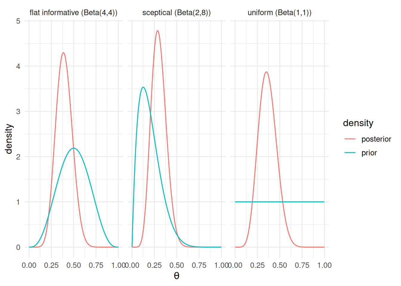
3. Assumptions
Bernoulli trials, exchangeable, conjugate beta prior. With no prior data on the response rate in this population, we carry all three priors through and compare decisions.
4. Conduct
Posterior summaries.
# A tibble: 3 × 5
# Rowwise:
  name                         post_mean ci_lo ci_hi p_gt_0_2
  <chr>                            <dbl> <dbl> <dbl>    <dbl>
1 uniform (Beta(1,1))              0.364 0.181 0.570    0.957
2 sceptical (Beta(2,8))            0.3   0.153 0.472    0.892
3 flat informative (Beta(4,4))     0.393 0.224 0.576    0.989
A frequentist analogue for comparison.
5. Conclude
With 7 responders out of 20, the posterior probability that the response rate exceeds 0.2 is 0.96 under a flat prior and 0.89 under a sceptical prior. A one-sided exact binomial test against p₀ = 0.2 gives p = 0.087.
All three priors point the same direction, but the strength of the conclusion depends on the prior. For a go/no-go decision, reporting the posterior probability of exceeding a decision threshold — along with its prior-sensitivity — is more decision-relevant than a p-value.
Common pitfalls
- Treating a 95% credible interval as a 95% confidence interval; they are calibrated for different inferences.
- Choosing a prior that pushes the posterior toward the desired decision and not reporting the sensitivity.
- Comparing a one-sided Bayesian tail probability to a two-sided p-value.
Further reading
- Spiegelhalter DJ, Abrams KR, Myles JP, Bayesian Approaches to Clinical Trials and Health-Care Evaluation.
- McElreath R, Statistical Rethinking, ch. 2–3.
Session info
R version 4.5.2 (2025-10-31 ucrt)
Platform: x86_64-w64-mingw32/x64
Running under: Windows 11 x64 (build 26200)

Matrix products: default
  LAPACK version 3.12.1

locale:
[1] LC_COLLATE=English_Germany.utf8  LC_CTYPE=English_Germany.utf8
[3] LC_MONETARY=English_Germany.utf8 LC_NUMERIC=C
[5] LC_TIME=English_Germany.utf8

time zone: Europe/Berlin
tzcode source: internal

attached base packages:
[1] stats     graphics  grDevices utils     datasets  methods   base

other attached packages:
 [1] lubridate_1.9.5 forcats_1.0.1   stringr_1.6.0   dplyr_1.2.1
 [5] purrr_1.2.2     readr_2.2.0     tidyr_1.3.2     tibble_3.3.1
 [9] ggplot2_4.0.3   tidyverse_2.0.0

loaded via a namespace (and not attached):
 [1] gtable_0.3.6       jsonlite_2.0.0     compiler_4.5.2     tidyselect_1.2.1
 [5] scales_1.4.0       yaml_2.3.12        fastmap_1.2.0      R6_2.6.1
 [9] labeling_0.4.3     generics_0.1.4     knitr_1.51         htmlwidgets_1.6.4
[13] pillar_1.11.1      RColorBrewer_1.1-3 tzdb_0.5.0         rlang_1.2.0
[17] utf8_1.2.6         stringi_1.8.7      xfun_0.57          S7_0.2.2
[21] otel_0.2.0         timechange_0.4.0   cli_3.6.6          withr_3.0.2
[25] magrittr_2.0.4     digest_0.6.39      grid_4.5.2         hms_1.1.4
[29] lifecycle_1.0.5    vctrs_0.7.3        evaluate_1.0.5     glue_1.8.1
[33] farver_2.1.2       rmarkdown_2.31     tools_4.5.2        pkgconfig_2.0.3
[37] htmltools_0.5.9