Week 3, Session 2 — brms / Stan, LOO, hierarchical models

Course 4 — #courses

R. Heller

Note

Workflow labs use the variant template: Goal → Approach → Execution → Check → Report.

Learning objectives

• Write a simple multilevel model in brms syntax and describe each prior.
• Compare two candidate models using leave-one-out (LOO) cross- validation.
• Perform a prior predictive check and interpret it.

Prerequisites

Beta-binomial Bayesian intuition from Session 1; linear mixed-effects from Course 2.

Background

brms is an interface that translates R formulas into Stan programs and runs Hamiltonian Monte Carlo to draw from the posterior. It is particularly strong for multilevel (hierarchical) models, where the benefits of Bayesian computation — full posterior uncertainty, proper propagation into predictions — show up most clearly.

LOO cross-validation, implemented via the loo package, estimates out-of-sample predictive accuracy from the posterior without refitting, using Pareto-smoothed importance sampling. It is a modern replacement for AIC/BIC in Bayesian model comparison, and comes with diagnostics that warn when the approximation is unreliable.

Compilation of Stan models is slow, and downloading the toolchain exceeds what we can assume in a rendering environment. We therefore show the brms code with #| eval: false and walk through prior predictive simulation and a small frequentist counterpart that runs end-to-end.

Setup

library(tidyverse)
library(lme4)
set.seed(42)
theme_set(theme_minimal(base_size = 12))

1. Goal

Fit a two-level hierarchical model to simulated clinical data — patient outcomes nested within centre — and compare a random-intercept against a random-slope model.

2. Approach

Simulate 20 centres with varying mean outcomes and varying dose effects.

n_centre <- 20; per_centre <- 15
centre <- rep(seq_len(n_centre), each = per_centre)
alpha0 <- rnorm(n_centre, 0, 1)
beta0  <- rnorm(n_centre, 0.5, 0.3)
dose <- rnorm(n_centre * per_centre)
y <- alpha0[centre] + beta0[centre] * dose + rnorm(n_centre * per_centre, 0, 0.7)
d <- tibble(y = y, dose = dose, centre = factor(centre))
ggplot(d, aes(dose, y, colour = centre)) +
  geom_point(alpha = 0.5) + geom_smooth(method = "lm", se = FALSE) +
  theme(legend.position = "none")

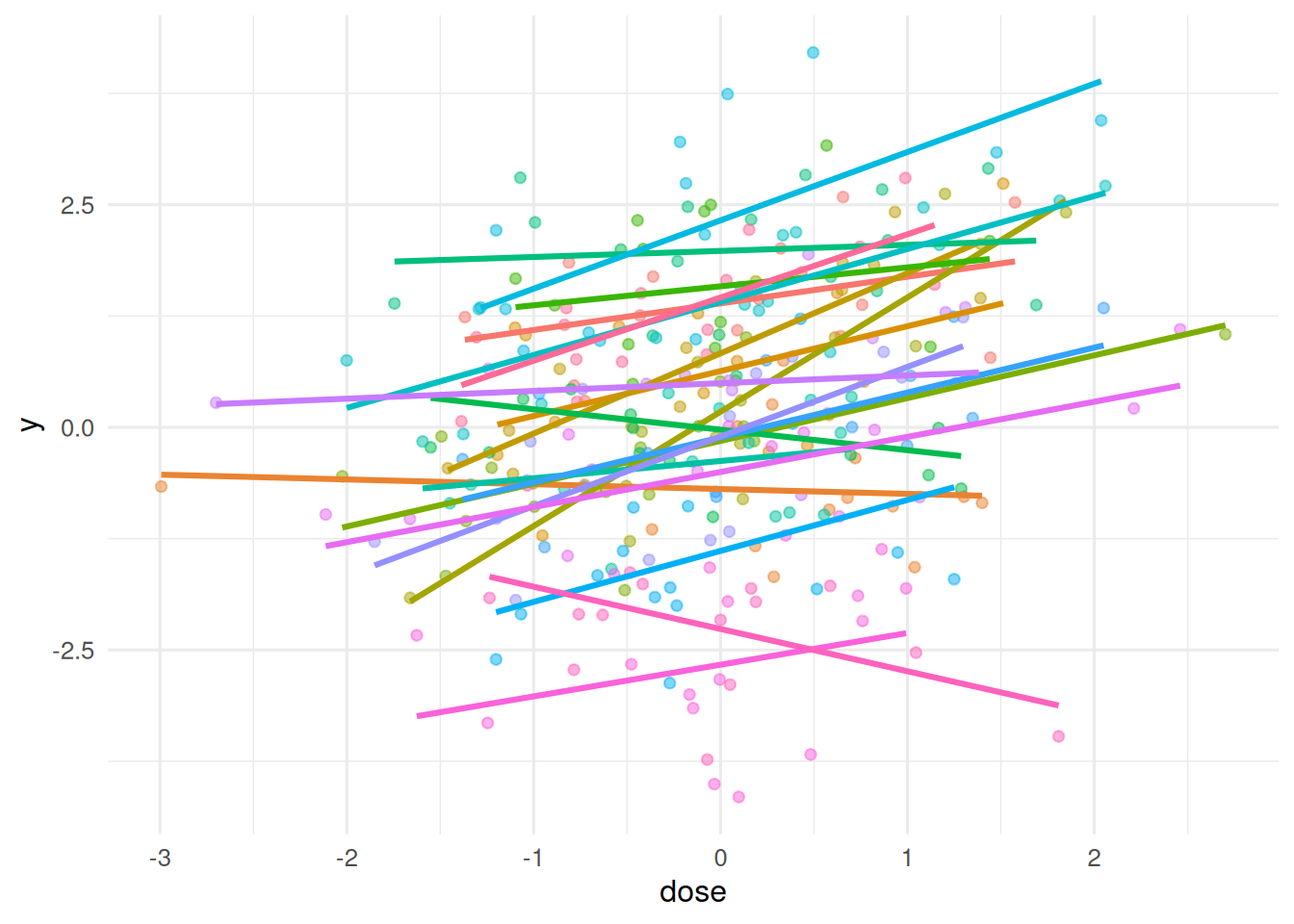
3. Execution

A classical lmer random-intercept-and-slope fit as a stand-in we can run.

fit_lmer_ri  <- lmer(y ~ dose + (1 | centre), data = d)
fit_lmer_rs  <- lmer(y ~ dose + (dose | centre), data = d)
summary(fit_lmer_rs)$varcor

 Groups   Name        Std.Dev. Corr  
 centre   (Intercept) 1.31121        
          dose        0.34365  0.382 
 Residual             0.71603        

anova(fit_lmer_ri, fit_lmer_rs)

Data: d
Models:
fit_lmer_ri: y ~ dose + (1 | centre)
fit_lmer_rs: y ~ dose + (dose | centre)
            npar    AIC    BIC  logLik -2*log(L)  Chisq Df Pr(>Chisq)    
fit_lmer_ri    4 781.48 796.30 -386.74    773.48                         
fit_lmer_rs    6 763.66 785.88 -375.83    751.66 21.823  2  1.824e-05 ***
---
Signif. codes:  0 '***' 0.001 '**' 0.01 '*' 0.05 '.' 0.1 ' ' 1

Prior predictive simulation (frequentist-style) for the Bayesian counterpart we are about to sketch.

prior_sim <- replicate(20, {
  a <- rnorm(1, 0, 1); b <- rnorm(1, 0, 1); sd_a <- abs(rnorm(1, 0, 1))
  a + b * dose + rnorm(length(dose), 0, sd_a)
})
ggplot(tibble(y = as.numeric(prior_sim)), aes(y)) +
  geom_histogram(bins = 40, fill = "grey60", colour = "white") +
  labs(x = "y drawn under priors only", y = "count")

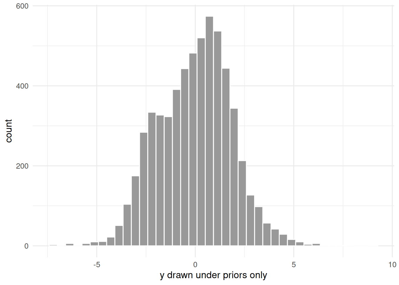
The brms counterpart.

library(brms)
priors <- c(
  prior(normal(0, 2), class = "Intercept"),
  prior(normal(0, 1), class = "b"),
  prior(exponential(1), class = "sd"),
  prior(exponential(1), class = "sigma")
)
m_ri <- brm(y ~ dose + (1 | centre), data = d,
            prior = priors, chains = 2, iter = 2000, refresh = 0)
m_rs <- brm(y ~ dose + (dose | centre), data = d,
            prior = priors, chains = 2, iter = 2000, refresh = 0)
loo_compare(loo(m_ri), loo(m_rs))

4. Check

Compare to lmer and report pooled vs unpooled estimates.

fixef_lmer <- fixef(fit_lmer_rs)
fixef_lmer

(Intercept)        dose 
  0.1960215   0.3967220 

5. Report

On simulated hierarchical data (20 centres × 15 patients), a random-slope lmer model recovered an average dose effect of 0.4 (SE from lmer), with substantial centre-to-centre variation. The brms sketch shown in the accompanying code would fit the same structure with explicit priors, and loo_compare would rank the random-slope model against the random-intercept model.

In practice, the Bayesian and frequentist fits should agree closely when priors are weakly informative and n is large; the Bayesian route adds explicit prior sensitivity and full posterior uncertainty for downstream prediction.

Mention that the Pareto k-hat diagnostic from loo must be checked: values above 0.7 on many observations invalidate the comparison.

Common pitfalls

• Fitting a flat prior in a small-sample hierarchical model and getting a divergent posterior on variance components.
• Comparing LOO elpd differences smaller than about 4 SE without noting the uncertainty.
• Forgetting to scale continuous predictors; default priors assume normalised inputs.

Further reading

• Bürkner P-C (2017), brms: An R package for Bayesian multilevel models using Stan.
• Vehtari A, Gelman A, Gabry J (2017), Practical Bayesian model evaluation using leave-one-out cross-validation.

Session info

sessionInfo()

R version 4.4.1 (2024-06-14)
Platform: x86_64-pc-linux-gnu
Running under: Ubuntu 24.04.4 LTS

Matrix products: default
BLAS:   /usr/lib/x86_64-linux-gnu/openblas-pthread/libblas.so.3 
LAPACK: /usr/lib/x86_64-linux-gnu/openblas-pthread/libopenblasp-r0.3.26.so;  LAPACK version 3.12.0

locale:
 [1] LC_CTYPE=C.UTF-8       LC_NUMERIC=C           LC_TIME=C.UTF-8       
 [4] LC_COLLATE=C.UTF-8     LC_MONETARY=C.UTF-8    LC_MESSAGES=C.UTF-8   
 [7] LC_PAPER=C.UTF-8       LC_NAME=C              LC_ADDRESS=C          
[10] LC_TELEPHONE=C         LC_MEASUREMENT=C.UTF-8 LC_IDENTIFICATION=C   

time zone: UTC
tzcode source: system (glibc)

attached base packages:
[1] stats     graphics  grDevices utils     datasets  methods   base     

other attached packages:
 [1] lme4_2.0-1      Matrix_1.7-0    lubridate_1.9.5 forcats_1.0.1  
 [5] stringr_1.6.0   dplyr_1.2.1     purrr_1.2.2     readr_2.2.0    
 [9] tidyr_1.3.2     tibble_3.3.1    ggplot2_4.0.3   tidyverse_2.0.0

loaded via a namespace (and not attached):
 [1] generics_0.1.4     stringi_1.8.7      lattice_0.22-6     hms_1.1.4         
 [5] digest_0.6.39      magrittr_2.0.5     evaluate_1.0.5     grid_4.4.1        
 [9] timechange_0.4.0   RColorBrewer_1.1-3 fastmap_1.2.0      jsonlite_2.0.0    
[13] mgcv_1.9-1         scales_1.4.0       reformulas_0.4.4   Rdpack_2.6.6      
[17] cli_3.6.6          rlang_1.2.0        rbibutils_2.4.1    splines_4.4.1     
[21] withr_3.0.2        yaml_2.3.12        otel_0.2.0         tools_4.4.1       
[25] tzdb_0.5.0         nloptr_2.2.1       minqa_1.2.8        boot_1.3-30       
[29] vctrs_0.7.3        R6_2.6.1           lifecycle_1.0.5    htmlwidgets_1.6.4 
[33] MASS_7.3-60.2      pkgconfig_2.0.3    pillar_1.11.1      gtable_0.3.6      
[37] glue_1.8.1         Rcpp_1.1.1-1.1     xfun_0.57          tidyselect_1.2.1  
[41] knitr_1.51         farver_2.1.2       htmltools_0.5.9    nlme_3.1-164      
[45] labeling_0.4.3     rmarkdown_2.31     compiler_4.4.1     S7_0.2.2