Week 3, Session 3 — Biomarker statistics (Youden, NRI, decision curves)

Course 4 — #courses

R. Heller

Note

Testing labs use the main template: Hypothesis → Visualise → Assumptions → Conduct → Conclude.

Learning objectives

• Compute ROC-AUC, Youden’s index, sensitivity, and specificity at the optimal cut-point.
• Compute a net reclassification index between two predictive models.
• Construct a decision curve and interpret net benefit at a range of threshold probabilities.

Prerequisites

Binary classification and ROC curves from Course 1; logistic regression.

Background

A candidate biomarker is not useful until it is tied to a decision. ROC-AUC summarises discrimination across all thresholds but is insensitive to where on the curve the action happens. Youden’s index (sensitivity + specificity − 1) picks the threshold that maximises the equal-weighted sum. The net reclassification index (NRI) quantifies whether a new model reclassifies cases and non-cases in the correct direction relative to a baseline. Decision curve analysis plots net benefit as a function of the threshold probability, and lets a reader compare strategies (“treat all”, “treat none”, “treat by model”) across a clinically relevant range.

Discrimination, calibration, and net benefit are three complementary axes. A biomarker with high AUC that is poorly calibrated can produce harmful decisions; a perfectly calibrated biomarker with low AUC gives no useful ranking. Reporting all three keeps the evaluation honest.

Decision curves are not hypothesis tests. They are a principled way to put a clinical question — what is the harm-to-benefit ratio of acting on this prediction? — into the analysis, and to see how the answer depends on that ratio.

Setup

library(tidyverse)
library(pROC)
library(MASS)
set.seed(42)
theme_set(theme_minimal(base_size = 12))

1. Hypothesis

Can a logistic model on Pima.tr (glucose, BMI, age) distinguish diabetic from non-diabetic patients well enough to support a screening decision?

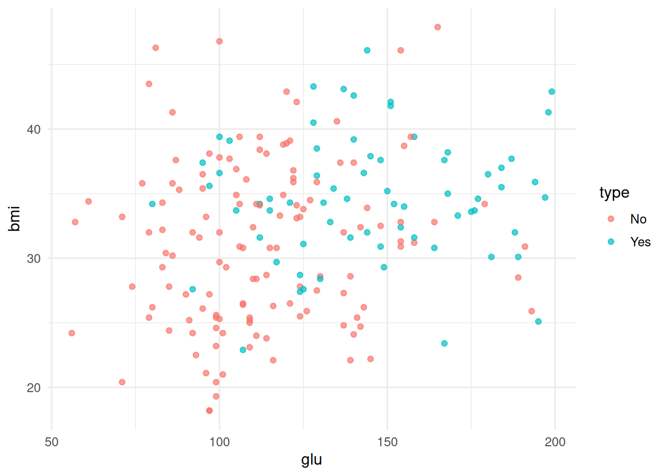
2. Visualise

d <- as_tibble(MASS::Pima.tr)
ggplot(d, aes(glu, bmi, colour = type)) + geom_point(alpha = 0.7)

3. Assumptions

Independence of observations; probability of diabetes is monotone in the linear predictor; no missingness.

4. Conduct

Fit a simple logistic regression and compute discrimination.

fit <- glm(type ~ glu + bmi + age, data = d, family = binomial())
d$p <- predict(fit, type = "response")
r  <- roc(d$type, d$p, direction = "<", quiet = TRUE)
auc(r)

Area under the curve: 0.8355

coords(r, "best", ret = c("threshold", "sensitivity", "specificity",
                          "youden"), transpose = FALSE)

  threshold sensitivity specificity   youden
1  0.267804   0.8676471   0.6969697 1.564617

NRI against a glucose-only baseline.

fit0 <- glm(type ~ glu, data = d, family = binomial())
p0 <- predict(fit0, type = "response")
p1 <- d$p
# Continuous NRI
case   <- d$type == "Yes"
nri_up <- mean(p1[case]  > p0[case])   - mean(p1[case]  < p0[case])
nri_dn <- mean(p1[!case] < p0[!case])  - mean(p1[!case] > p0[!case])
nri <- nri_up + nri_dn
c(nri_cases = nri_up, nri_noncases = nri_dn, nri_total = nri)

   nri_cases nri_noncases    nri_total 
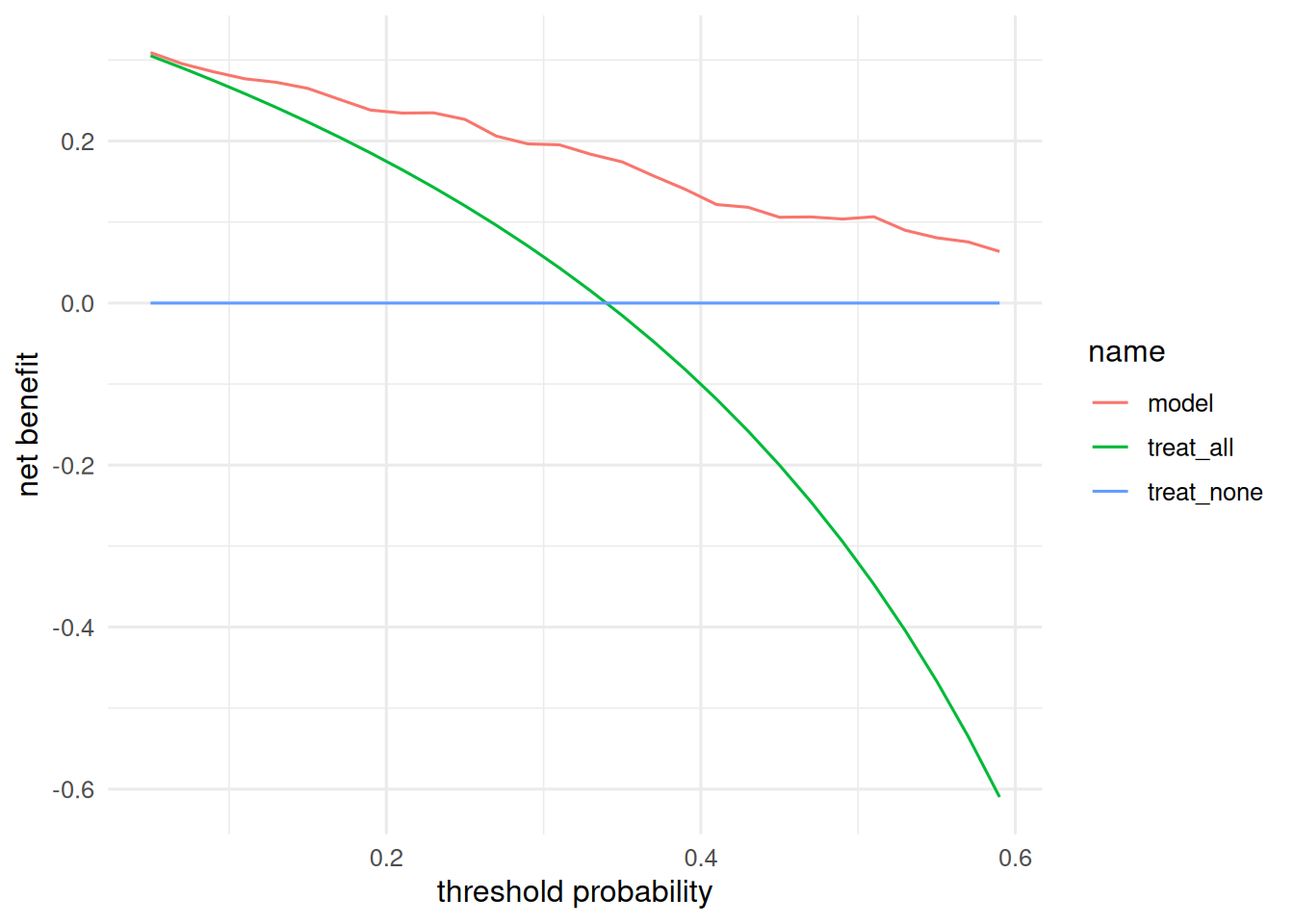
   0.2941176    0.2878788    0.5819964 

A manual decision curve.

thr <- seq(0.05, 0.6, by = 0.02)
dca <- sapply(thr, function(t) {
  treat <- p1 > t
  tp <- sum(treat &  case); fp <- sum(treat & !case); N <- length(case)
  tp / N - (fp / N) * (t / (1 - t))
})
nb_all <- sapply(thr, function(t) {
  tp <- sum(case); fp <- sum(!case); N <- length(case)
  tp / N - (fp / N) * (t / (1 - t))
})
tibble(threshold = thr, model = dca, treat_all = nb_all, treat_none = 0) |>
  pivot_longer(-threshold) |>
  ggplot(aes(threshold, value, colour = name)) + geom_line() +
  labs(x = "threshold probability", y = "net benefit")

5. Concluding statement

A logistic model using glucose, BMI, and age discriminated diabetic from non-diabetic patients in MASS::Pima.tr with AUC 0.835. The Youden-optimal cut-point occurred at a predicted probability of 0.27. Adding BMI and age to a glucose-only baseline produced an NRI of 0.58; the decision curve showed net benefit above “treat all” for threshold probabilities from roughly 0.15 to 0.5.

Decision curves give the clinical context: if the decision to intervene at, say, p = 0.2 is under discussion, the model is useful; at p = 0.05 or p = 0.7, it is barely distinguishable from treat-all or treat-none.

If time, show bootstrap CIs for AUC with pROC::ci.auc and for net benefit with resampling.

Common pitfalls

• Reporting AUC without calibration or decision curves.
• Computing NRI with a categorical risk cut-point and failing to disclose the cut-off.
• Using the same data to develop and evaluate the biomarker (apparent performance).

Further reading

• Pencina MJ, D’Agostino RB Sr, et al. (2008), Evaluating the added predictive ability of a new marker.
• Vickers AJ, Elkin EB (2006), Decision curve analysis.

Session info

sessionInfo()

R version 4.4.1 (2024-06-14)
Platform: x86_64-pc-linux-gnu
Running under: Ubuntu 24.04.4 LTS

Matrix products: default
BLAS:   /usr/lib/x86_64-linux-gnu/openblas-pthread/libblas.so.3 
LAPACK: /usr/lib/x86_64-linux-gnu/openblas-pthread/libopenblasp-r0.3.26.so;  LAPACK version 3.12.0

locale:
 [1] LC_CTYPE=C.UTF-8       LC_NUMERIC=C           LC_TIME=C.UTF-8       
 [4] LC_COLLATE=C.UTF-8     LC_MONETARY=C.UTF-8    LC_MESSAGES=C.UTF-8   
 [7] LC_PAPER=C.UTF-8       LC_NAME=C              LC_ADDRESS=C          
[10] LC_TELEPHONE=C         LC_MEASUREMENT=C.UTF-8 LC_IDENTIFICATION=C   

time zone: UTC
tzcode source: system (glibc)

attached base packages:
[1] stats     graphics  grDevices utils     datasets  methods   base     

other attached packages:
 [1] MASS_7.3-60.2   pROC_1.19.0.1   lubridate_1.9.5 forcats_1.0.1  
 [5] stringr_1.6.0   dplyr_1.2.1     purrr_1.2.2     readr_2.2.0    
 [9] tidyr_1.3.2     tibble_3.3.1    ggplot2_4.0.3   tidyverse_2.0.0

loaded via a namespace (and not attached):
 [1] gtable_0.3.6       jsonlite_2.0.0     compiler_4.4.1     Rcpp_1.1.1-1.1    
 [5] tidyselect_1.2.1   scales_1.4.0       yaml_2.3.12        fastmap_1.2.0     
 [9] R6_2.6.1           labeling_0.4.3     generics_0.1.4     knitr_1.51        
[13] htmlwidgets_1.6.4  pillar_1.11.1      RColorBrewer_1.1-3 tzdb_0.5.0        
[17] rlang_1.2.0        stringi_1.8.7      xfun_0.57          S7_0.2.2          
[21] otel_0.2.0         timechange_0.4.0   cli_3.6.6          withr_3.0.2       
[25] magrittr_2.0.5     digest_0.6.39      grid_4.4.1         hms_1.1.4         
[29] lifecycle_1.0.5    vctrs_0.7.3        evaluate_1.0.5     glue_1.8.1        
[33] farver_2.1.2       rmarkdown_2.31     tools_4.4.1        pkgconfig_2.0.3   
[37] htmltools_0.5.9