Week 3, Session 4 — Survival ML (random survival forest, DeepSurv)

Course 4 — #courses

R. Heller

Note

Workflow labs use the variant template: Goal → Approach → Execution → Check → Report.

Learning objectives

• Fit a random survival forest and interpret its variable importance and risk stratification.
• Describe the DeepSurv architecture conceptually and when it is preferred over the forest.
• Compare against a Cox model on the same features.

Prerequisites

Cox regression and censoring from Course 2.

Background

Survival analysis deals with time-to-event data in the presence of censoring. The Cox proportional-hazards model is the workhorse linear method; random survival forests (RSF) extend the idea of random forests to right-censored outcomes, using a log-rank split rule and Harrell’s concordance as the default fit criterion. They handle nonlinearities and interactions automatically and are a good first nonparametric benchmark.

DeepSurv is a neural-network generalisation of the Cox partial likelihood: the linear predictor is replaced by a feed-forward network. In small biomedical datasets it rarely beats a well-tuned RSF or a Cox model with splines, but the approach scales to large cohorts and to inputs where a representation must be learned.

Evaluation of survival models uses time-integrated concordance (Harrell’s C), the integrated Brier score, and — increasingly — decision curves at a clinically relevant horizon. Reporting only C on a single test set is weak evidence.

Setup

library(tidyverse)
library(survival)
library(randomForestSRC)
set.seed(42)
theme_set(theme_minimal(base_size = 12))

1. Goal

Fit an RSF on survival::pbc and compare to a Cox model using Harrell’s concordance.

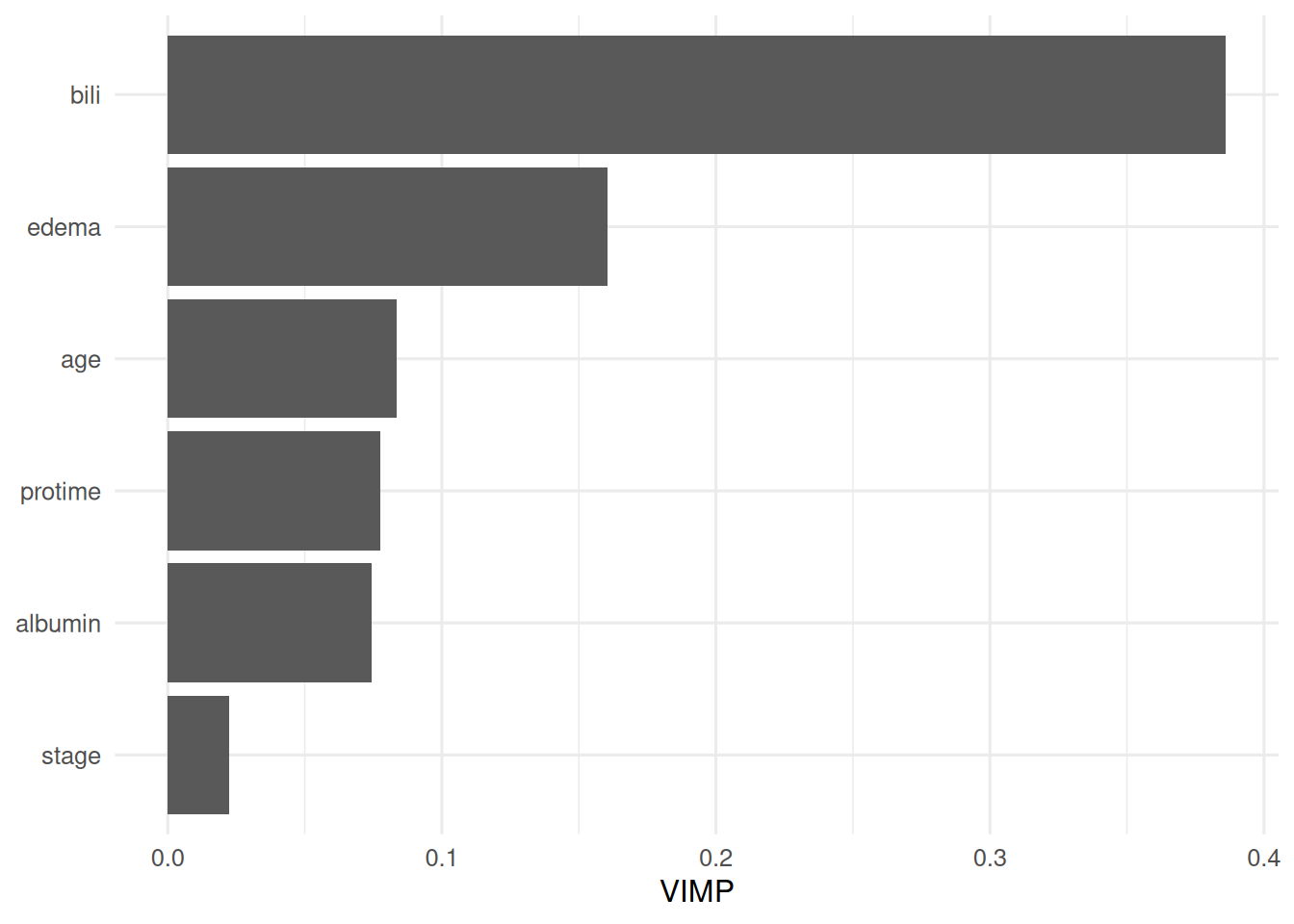
2. Approach

d <- survival::pbc |>
  as_tibble() |>
  drop_na(bili, albumin, age, edema, protime, stage) |>
  mutate(status = ifelse(status == 2, 1, 0))

ggplot(d, aes(time / 365.25, fill = factor(status))) +
  geom_histogram(bins = 30, alpha = 0.7, position = "identity") +
  labs(x = "follow-up (years)", y = "count", fill = "event")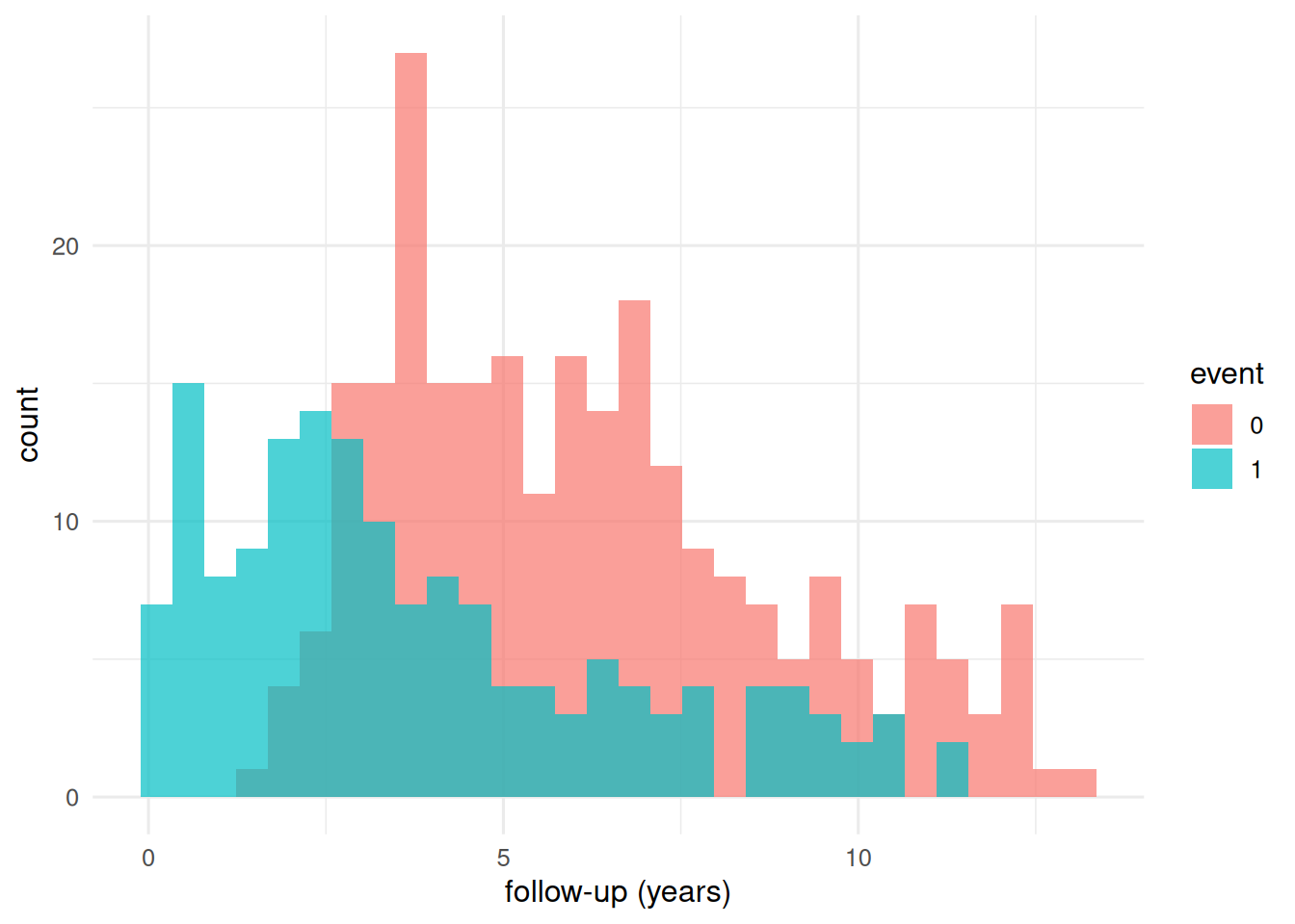

3. Execution

fit_cox <- coxph(Surv(time, status) ~ bili + albumin + age + edema +
                   protime + stage, data = d)
fit_rsf <- rfsrc(Surv(time, status) ~ bili + albumin + age + edema +
                   protime + stage,
                 data = as.data.frame(d), ntree = 500,
                 importance = TRUE)
fit_rsf

                         Sample size: 410
                    Number of deaths: 156
                     Number of trees: 500
           Forest terminal node size: 15
       Average no. of terminal nodes: 19.574
No. of variables tried at each split: 3
              Total no. of variables: 6
       Resampling used to grow trees: swor
    Resample size used to grow trees: 259
                            Analysis: RSF
                              Family: surv
                      Splitting rule: logrank *random*
       Number of random split points: 10
                          (OOB) CRPS: 505.07481851
             (OOB) standardized CRPS: 0.12051415
   (OOB) Requested performance error: 0.18039411

tibble(var = names(fit_rsf$importance),
       imp = as.numeric(fit_rsf$importance)) |>
  arrange(desc(imp)) |>
  ggplot(aes(reorder(var, imp), imp)) +
  geom_col() + coord_flip() + labs(x = NULL, y = "VIMP")

4. Check

Compare concordance on held-out data.

idx <- sample(nrow(d), 0.7 * nrow(d))
tr <- d[idx, ]; te <- d[-idx, ]
cox2 <- coxph(Surv(time, status) ~ bili + albumin + age + edema +
                protime + stage, data = tr)
rsf2 <- rfsrc(Surv(time, status) ~ bili + albumin + age + edema +
                protime + stage,
              data = as.data.frame(tr), ntree = 500)
c_cox <- survival::concordance(cox2, newdata = te)$concordance
p_rsf <- predict(rsf2, newdata = as.data.frame(te))$predicted
c_rsf <- survival::concordance(Surv(te$time, te$status) ~ p_rsf,
                               reverse = TRUE)$concordance
c(cox = c_cox, rsf = c_rsf)

      cox       rsf 
0.7854077 0.8071531 

DeepSurv conceptual sketch.

library(torch)
# A DeepSurv-style loss computes the partial log-likelihood on the
# sorted risk set. The network output h(x) replaces the Cox linear
# predictor; the loss is  -(sum_{i:event}  h(x_i) - log sum_{j in R_i} exp(h(x_j))).
deepsurv_loss <- function(risk, time, event) {
  ord <- order(time, decreasing = TRUE)
  risk <- risk[ord]; event <- event[ord]
  log_cumsum <- torch_logcumsumexp(risk, dim = 1)
  -torch_sum(event * (risk - log_cumsum)) / torch_sum(event)
}

5. Report

On survival::pbc, a random survival forest achieved test concordance 0.807 compared with 0.785 for a multivariable Cox model. Bilirubin, albumin, and age dominated VIMP. A DeepSurv network with the partial-likelihood loss would be the natural next step on a larger cohort.

On this sample size, the RSF and Cox model are close; on larger datasets with nonlinearities, the forest often pulls ahead.

Mention that randomForestSRC::vimp has a permutation variant worth preferring for correlated predictors.

Common pitfalls

• Treating the Cox proportional-hazards assumption as always met; it often is not, and the RSF is more robust to violation.
• Comparing models without the same censoring distribution in the test set.
• Reporting only C without a calibration or decision curve at the horizon of interest.

Further reading

• Ishwaran H et al. (2008), Random survival forests.
• Katzman JL et al. (2018), DeepSurv: Personalized treatment recommender system using a Cox proportional hazards deep neural network.

Session info

sessionInfo()

R version 4.4.1 (2024-06-14)
Platform: x86_64-pc-linux-gnu
Running under: Ubuntu 24.04.4 LTS

Matrix products: default
BLAS:   /usr/lib/x86_64-linux-gnu/openblas-pthread/libblas.so.3 
LAPACK: /usr/lib/x86_64-linux-gnu/openblas-pthread/libopenblasp-r0.3.26.so;  LAPACK version 3.12.0

locale:
 [1] LC_CTYPE=C.UTF-8       LC_NUMERIC=C           LC_TIME=C.UTF-8       
 [4] LC_COLLATE=C.UTF-8     LC_MONETARY=C.UTF-8    LC_MESSAGES=C.UTF-8   
 [7] LC_PAPER=C.UTF-8       LC_NAME=C              LC_ADDRESS=C          
[10] LC_TELEPHONE=C         LC_MEASUREMENT=C.UTF-8 LC_IDENTIFICATION=C   

time zone: UTC
tzcode source: system (glibc)

attached base packages:
[1] stats     graphics  grDevices utils     datasets  methods   base     

other attached packages:
 [1] randomForestSRC_3.6.2 survival_3.6-4        lubridate_1.9.5      
 [4] forcats_1.0.1         stringr_1.6.0         dplyr_1.2.1          
 [7] purrr_1.2.2           readr_2.2.0           tidyr_1.3.2          
[10] tibble_3.3.1          ggplot2_4.0.3         tidyverse_2.0.0      

loaded via a namespace (and not attached):
 [1] Matrix_1.7-0       gtable_0.3.6       jsonlite_2.0.0     compiler_4.4.1    
 [5] tidyselect_1.2.1   parallel_4.4.1     DiagrammeR_1.0.12  splines_4.4.1     
 [9] scales_1.4.0       yaml_2.3.12        fastmap_1.2.0      lattice_0.22-6    
[13] R6_2.6.1           labeling_0.4.3     generics_0.1.4     knitr_1.51        
[17] visNetwork_2.1.4   htmlwidgets_1.6.4  pillar_1.11.1      RColorBrewer_1.1-3
[21] tzdb_0.5.0         rlang_1.2.0        stringi_1.8.7      xfun_0.57         
[25] S7_0.2.2           otel_0.2.0         timechange_0.4.0   cli_3.6.6         
[29] withr_3.0.2        magrittr_2.0.5     digest_0.6.39      grid_4.4.1        
[33] hms_1.1.4          data.tree_1.2.0    lifecycle_1.0.5    vctrs_0.7.3       
[37] evaluate_1.0.5     glue_1.8.1         farver_2.1.2       rmarkdown_2.31    
[41] tools_4.4.1        pkgconfig_2.0.3    htmltools_0.5.9