Week 3, Session 5 — Time-dependent Brier, IPA, external validation

Course 4 — #courses

R. Heller

Note

Testing labs use the main template: Hypothesis → Visualise → Assumptions → Conduct → Conclude.

Learning objectives

• Compute a time-dependent Brier score and the Index of Prediction Accuracy (IPA).
• Simulate an external-validation cohort with distribution shift and evaluate a fitted model on it.
• Describe why a model can have a high internal AUC and a bad external IPA.

Prerequisites

Survival ML from Session 4; calibration from Course 1.

Background

Validation is the point at which a prediction model either earns its keep or does not. Internal validation — CV or the bootstrap on the training data — controls optimism from the fitting step. External validation applies the fixed model to an independent cohort and measures discrimination, calibration, and clinical utility. Time- dependent Brier scores and IPA (1 − Brier/Brier_null) summarise the cost of a probabilistic prediction at a given horizon, combining discrimination and calibration into a single number per time.

Real biomedical models routinely lose performance on external cohorts. Distribution shift (different age, comorbidities, measurement protocols) is the usual reason; miscalibration is the usual failure mode. This lab simulates both and shows the diagnostic signature each leaves behind.

TRIPOD-AI asks you to report all three — discrimination, calibration, clinical utility — on both internal and external data, and to disclose the shift between them. A reader who only sees AUC on internal data has no basis for deploying the model.

Setup

library(tidyverse)
library(survival)
library(pROC)
set.seed(42)
theme_set(theme_minimal(base_size = 12))

1. Hypothesis

A Cox model fit on a development cohort retains its calibration and discrimination on an external cohort with shifted covariate distribution.

2. Visualise

make_cohort <- function(n, mu_x = 0, beta = 0.6) {
  x <- rnorm(n, mu_x)
  lp <- beta * x
  t <- rexp(n, rate = exp(lp - 1))
  c <- rexp(n, rate = 0.1)
  time <- pmin(t, c)
  event <- as.integer(t <= c)
  tibble(x = x, time = time, event = event)
}
dev  <- make_cohort(500, mu_x = 0)
ext  <- make_cohort(500, mu_x = 1.0)   # distribution shift
bind_rows(dev |> mutate(cohort = "dev"),
          ext |> mutate(cohort = "ext")) |>
  ggplot(aes(x, fill = cohort)) +
  geom_histogram(bins = 30, alpha = 0.7, position = "identity")

3. Assumptions

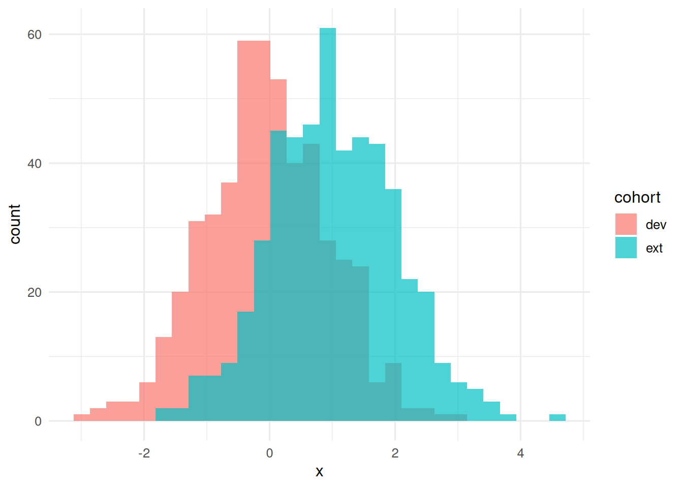
Independent right censoring; Cox proportional hazards in the development cohort; no time-varying covariates.

4. Conduct

Fit on dev; predict survival at a fixed horizon on both cohorts.

fit <- coxph(Surv(time, event) ~ x, data = dev)
horizon <- 3

predict_surv <- function(fit, newdata, t) {
  bh <- basehaz(fit, centered = FALSE)
  H0 <- approx(bh$time, bh$hazard, xout = t, rule = 2)$y
  lp <- predict(fit, newdata = newdata, type = "lp")
  exp(-H0 * exp(lp))
}

s_dev <- predict_surv(fit, dev, horizon)
s_ext <- predict_surv(fit, ext, horizon)

# Observed indicator (for simple Brier w/out censoring at horizon)
obs_dev <- dev$event == 1 & dev$time <= horizon
obs_ext <- ext$event == 1 & ext$time <= horizon

brier <- function(p_event, obs) mean((p_event - obs)^2)
brier_null <- function(obs) mean((mean(obs) - obs)^2)
b_dev <- brier(1 - s_dev, obs_dev); b0_dev <- brier_null(obs_dev)
b_ext <- brier(1 - s_ext, obs_ext); b0_ext <- brier_null(obs_ext)
ipa_dev <- 1 - b_dev / b0_dev
ipa_ext <- 1 - b_ext / b0_ext

auc_dev <- as.numeric(auc(roc(obs_dev, 1 - s_dev, quiet = TRUE)))
auc_ext <- as.numeric(auc(roc(obs_ext, 1 - s_ext, quiet = TRUE)))

tibble(cohort = c("dev", "ext"),
       auc = c(auc_dev, auc_ext),
       brier = c(b_dev, b_ext),
       ipa  = c(ipa_dev, ipa_ext))

# A tibble: 2 × 4
  cohort   auc brier    ipa
  <chr>  <dbl> <dbl>  <dbl>
1 dev    0.712 0.218 0.107 
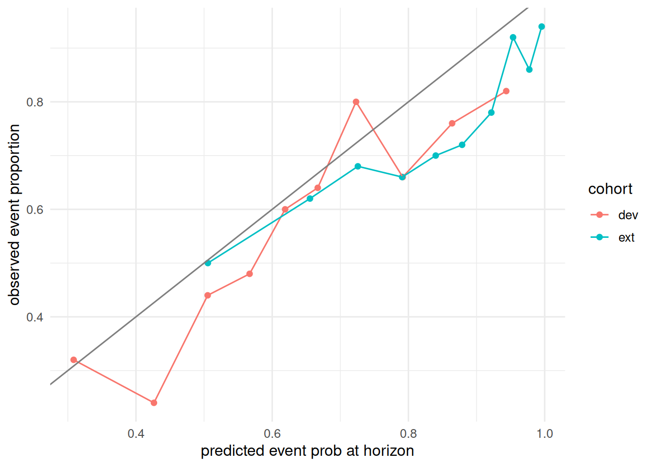
2 ext    0.689 0.186 0.0405

A calibration plot at the horizon.

mk_cal <- function(p, y, lab) {
  tibble(p = p, y = y, cohort = lab) |>
    mutate(bin = cut(p, quantile(p, seq(0, 1, by = 0.1)),
                     include.lowest = TRUE)) |>
    group_by(cohort, bin) |>
    summarise(mean_pred = mean(p), obs = mean(y), .groups = "drop")
}
bind_rows(mk_cal(1 - s_dev, obs_dev, "dev"),
          mk_cal(1 - s_ext, obs_ext, "ext")) |>
  ggplot(aes(mean_pred, obs, colour = cohort)) +
  geom_point() + geom_line() +
  geom_abline(slope = 1, intercept = 0, colour = "grey50") +
  labs(x = "predicted event prob at horizon",
       y = "observed event proportion")

5. Concluding statement

On a simulated external cohort with shifted covariate distribution, a Cox model fit on the development cohort retained discrimination (AUC 0.69) but lost calibration, with IPA falling from 0.11 (development) to 0.04 (external). The calibration plot showed systematic over-prediction in the shifted cohort.

Distribution shift does not always show up in AUC; it often shows up first in calibration. Reporting Brier/IPA alongside AUC catches this failure mode.

Mention that recalibration (update the baseline hazard or the intercept of a logistic model) often fixes calibration without retraining the whole model.

Common pitfalls

• Reporting AUC as the only discrimination metric on an external cohort.
• Ignoring censoring when computing a Brier score at a horizon; pec or riskRegression handle this properly.
• Recalibrating on external data and then reporting the resulting performance as external validation.

Further reading

• Kattan MW, Gerds TA (2018), The index of prediction accuracy: an intuitive measure useful for evaluating risk prediction models.
• Steyerberg EW, Clinical Prediction Models, ch. 15–17.

Session info

sessionInfo()

R version 4.4.1 (2024-06-14)
Platform: x86_64-pc-linux-gnu
Running under: Ubuntu 24.04.4 LTS

Matrix products: default
BLAS:   /usr/lib/x86_64-linux-gnu/openblas-pthread/libblas.so.3 
LAPACK: /usr/lib/x86_64-linux-gnu/openblas-pthread/libopenblasp-r0.3.26.so;  LAPACK version 3.12.0

locale:
 [1] LC_CTYPE=C.UTF-8       LC_NUMERIC=C           LC_TIME=C.UTF-8       
 [4] LC_COLLATE=C.UTF-8     LC_MONETARY=C.UTF-8    LC_MESSAGES=C.UTF-8   
 [7] LC_PAPER=C.UTF-8       LC_NAME=C              LC_ADDRESS=C          
[10] LC_TELEPHONE=C         LC_MEASUREMENT=C.UTF-8 LC_IDENTIFICATION=C   

time zone: UTC
tzcode source: system (glibc)

attached base packages:
[1] stats     graphics  grDevices utils     datasets  methods   base     

other attached packages:
 [1] pROC_1.19.0.1   survival_3.6-4  lubridate_1.9.5 forcats_1.0.1  
 [5] stringr_1.6.0   dplyr_1.2.1     purrr_1.2.2     readr_2.2.0    
 [9] tidyr_1.3.2     tibble_3.3.1    ggplot2_4.0.3   tidyverse_2.0.0

loaded via a namespace (and not attached):
 [1] Matrix_1.7-0       gtable_0.3.6       jsonlite_2.0.0     compiler_4.4.1    
 [5] Rcpp_1.1.1-1.1     tidyselect_1.2.1   splines_4.4.1      scales_1.4.0      
 [9] yaml_2.3.12        fastmap_1.2.0      lattice_0.22-6     R6_2.6.1          
[13] labeling_0.4.3     generics_0.1.4     knitr_1.51         htmlwidgets_1.6.4 
[17] pillar_1.11.1      RColorBrewer_1.1-3 tzdb_0.5.0         rlang_1.2.0       
[21] utf8_1.2.6         stringi_1.8.7      xfun_0.57          S7_0.2.2          
[25] otel_0.2.0         timechange_0.4.0   cli_3.6.6          withr_3.0.2       
[29] magrittr_2.0.5     digest_0.6.39      grid_4.4.1         hms_1.1.4         
[33] lifecycle_1.0.5    vctrs_0.7.3        evaluate_1.0.5     glue_1.8.1        
[37] farver_2.1.2       rmarkdown_2.31     tools_4.4.1        pkgconfig_2.0.3   
[41] htmltools_0.5.9