Week 4, Session 4 — FDR, knockoffs, replication crisis
Course 4 — #courses
Note
Workflow labs use the variant template: Goal → Approach → Execution → Check → Report.
Learning objectives
- Simulate p-values under a mixture of null and alternative hypotheses and apply Benjamini–Hochberg FDR control.
- Describe the knockoff filter in words and explain what “exchangeable” means in that context.
- Connect FDR discipline to the replication crisis in biomedicine.
Prerequisites
Multiple-testing basics from Course 1.
Background
Multiple-testing corrections come in two families: family-wise error rate (Bonferroni, Holm) control the probability of any false discovery; false-discovery rate methods (Benjamini–Hochberg, Storey’s q-value) control the proportion of false discoveries among the discoveries. FDR is the appropriate target for the typical screen with thousands of simultaneous tests and a tolerance for some false positives on the shortlist.
Knockoffs are a newer idea that replace the classical p-value route entirely. For each feature a “knockoff” variable is constructed that matches the feature’s joint distribution with other features but is conditionally independent of the outcome. A statistic comparing the original and the knockoff then controls the FDR without distributional assumptions on the test statistic, provided the knockoffs are exchangeable.
The replication crisis in biomedicine is not usually a failure of FDR in the technical sense; it is usually a failure to control researcher degrees of freedom — the multiple analyses that precede the reported test. No post-hoc correction can rescue a flexible, undocumented workflow.
Pre-registration, code availability, and transparent reporting discipline the part of the pipeline that FDR cannot. They are not optional extras.
Setup
1. Goal
Simulate 1 000 tests, most null and a few alternative, and compare uncorrected, Bonferroni, and BH discovery sets.
2. Approach
m <- 1000
m1 <- 50
is_alt <- c(rep(TRUE, m1), rep(FALSE, m - m1))
mu <- ifelse(is_alt, 3, 0)
z <- rnorm(m, mu, 1)
p <- 2 * (1 - pnorm(abs(z)))

tibble(p = p, is_alt = is_alt) |>
  ggplot(aes(p, fill = is_alt)) +
  geom_histogram(bins = 40, position = "identity", alpha = 0.7) +
  labs(x = "p-value", y = "count")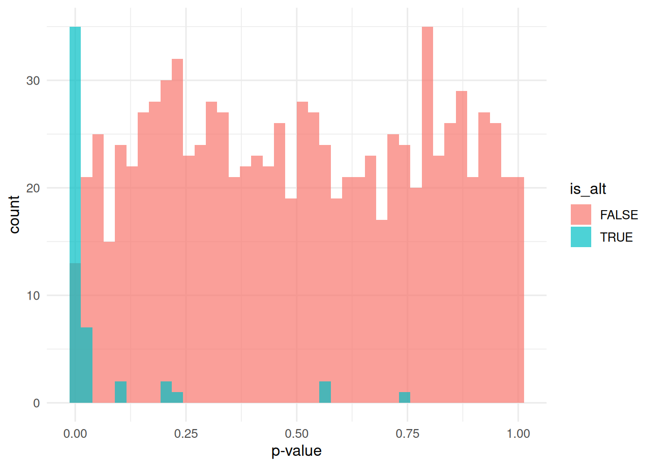
3. Execution
bonf <- p.adjust(p, method = "bonferroni")
bh   <- p.adjust(p, method = "BH")

res <- tibble(
  method = c("raw p<0.05", "Bonferroni<0.05", "BH q<0.05"),
  discovered  = c(sum(p < 0.05), sum(bonf < 0.05), sum(bh < 0.05)),
  true_pos    = c(sum(p[is_alt] < 0.05),
                  sum(bonf[is_alt] < 0.05),
                  sum(bh[is_alt] < 0.05)),
  false_pos   = c(sum(p[!is_alt] < 0.05),
                  sum(bonf[!is_alt] < 0.05),
                  sum(bh[!is_alt] < 0.05))
) |> mutate(fdp = false_pos / pmax(discovered, 1))
res
# A tibble: 3 × 5
method discovered true_pos false_pos fdp
<chr> <int> <int> <int> <dbl>
1 raw p<0.05 86 42 44 0.512
2 Bonferroni<0.05 9 9 0 0
3 BH q<0.05 23 21 2 0.08704. Check
Knockoff discussion — the idea, in words.
library(knockoff)
# For a linear regression y ~ X with X gaussian, construct
# Xk matching the second-order structure of X but conditionally
# independent of y given X. Then fit a penalised regression on
# [X, Xk]; the per-feature statistic W_j = |beta_j| - |beta_{j+p}|
# controls the FDR among selected features.
ko <- knockoff.filter(X, y, fdr = 0.1)
ko$selected
5. Report
On 1 000 simulated tests (50 alternative, 950 null), raw p-value cut-off at 0.05 produced 86 discoveries with a false-discovery proportion of 0.51. Bonferroni correction produced 9 discoveries; the BH procedure at q < 0.05 produced 23 with a false-discovery proportion of 0.09.
Knockoffs would give a similar FDR guarantee via a different route, and would remain valid under correlation between features provided the joint distribution can be modelled.
Common pitfalls
- Reporting nominal p < 0.05 cut-offs in a high-dimensional screen.
- Applying BH to a set of tests that are not approximately independent or positive-dependent.
- Treating knockoffs as a drop-in for p-values without checking the exchangeability assumption.
Further reading
- Benjamini Y, Hochberg Y (1995), Controlling the false discovery rate: A practical and powerful approach to multiple testing.
- Barber RF, Candès EJ (2015), Controlling the false discovery rate via knockoffs.
- Ioannidis JPA (2005), Why most published research findings are false.
Session info
R version 4.5.2 (2025-10-31 ucrt)
Platform: x86_64-w64-mingw32/x64
Running under: Windows 11 x64 (build 26200)

Matrix products: default
  LAPACK version 3.12.1

locale:
[1] LC_COLLATE=English_Germany.utf8  LC_CTYPE=English_Germany.utf8
[3] LC_MONETARY=English_Germany.utf8 LC_NUMERIC=C
[5] LC_TIME=English_Germany.utf8

time zone: Europe/Berlin
tzcode source: internal

attached base packages:
[1] stats     graphics  grDevices utils     datasets  methods   base

other attached packages:
 [1] lubridate_1.9.5 forcats_1.0.1   stringr_1.6.0   dplyr_1.2.1
 [5] purrr_1.2.2     readr_2.2.0     tidyr_1.3.2     tibble_3.3.1
 [9] ggplot2_4.0.3   tidyverse_2.0.0

loaded via a namespace (and not attached):
 [1] gtable_0.3.6       jsonlite_2.0.0     compiler_4.5.2     tidyselect_1.2.1
 [5] scales_1.4.0       yaml_2.3.12        fastmap_1.2.0      R6_2.6.1
 [9] labeling_0.4.3     generics_0.1.4     knitr_1.51         htmlwidgets_1.6.4
[13] pillar_1.11.1      RColorBrewer_1.1-3 tzdb_0.5.0         rlang_1.2.0
[17] utf8_1.2.6         stringi_1.8.7      xfun_0.57          S7_0.2.2
[21] otel_0.2.0         timechange_0.4.0   cli_3.6.6          withr_3.0.2
[25] magrittr_2.0.4     digest_0.6.39      grid_4.5.2         hms_1.1.4
[29] lifecycle_1.0.5    vctrs_0.7.3        evaluate_1.0.5     glue_1.8.1
[33] farver_2.1.2       rmarkdown_2.31     tools_4.5.2        pkgconfig_2.0.3
[37] htmltools_0.5.9