---
title: "Zero-knowledge proofs and strategic verification"
description: "Analyse zero-knowledge proof protocols as strategic games between prover and verifier. Model completeness, soundness, and zero-knowledge as equilibrium properties and explore interactive proofs for graph colouring."
author: "Raban Heller"
date: 2026-05-08
date-modified: 2026-05-08
categories:
- cryptography-and-gt
- zero-knowledge-proofs
- interactive-proofs
- verification-games
keywords: ["zero-knowledge-proofs", "interactive-proofs", "prover-verifier game", "completeness", "soundness", "graph colouring", "strategic verification"]
labels: ["cryptography-and-gt", "zero-knowledge", "verification"]
tier: 1
bibliography: ../../../references.bib
vgwort: "TODO_VGWORT_cryptography-and-gt_zero-knowledge-proofs-games"
image: thumbnail.png
image-alt: "Line plot showing the soundness error probability decreasing exponentially with the number of protocol rounds in a zero-knowledge proof verification game, rendered using the Okabe-Ito palette."
citation:
type: webpage
url: https://cttir.github.io/equilibria/tutorials/cryptography-and-gt/zero-knowledge-proofs-games/
license: "CC BY-SA 4.0"
draft: false
has_static_fig: true
has_interactive_fig: true
has_shiny_app: false
---
```{r}
#| label: setup
#| include: false
library(ggplot2)
library(dplyr)
library(tidyr)
library(plotly)
okabe_ito <- c("#E69F00", "#56B4E9", "#009E73", "#F0E442",
"#0072B2", "#D55E00", "#CC79A7", "#999999")
theme_publication <- function(base_size = 12) {
theme_minimal(base_size = base_size) +
theme(plot.title = element_text(size = base_size * 1.2, face = "bold"),
plot.subtitle = element_text(size = base_size * 0.9, color = "grey40"),
axis.line = element_line(color = "grey30", linewidth = 0.3),
panel.grid.minor = element_blank(), legend.position = "bottom",
plot.margin = margin(10, 10, 10, 10))
}
```
## Introduction and motivation
Zero-knowledge proofs represent one of the most remarkable achievements at the intersection of cryptography and theoretical computer science. Introduced by Goldwasser, Micali, and Rackoff in the 1980s, they allow a prover to convince a verifier that a statement is true without revealing any information beyond the truth of the statement itself. This seemingly paradoxical capability has profound implications for privacy, authentication, and secure computation. What is less widely appreciated is that zero-knowledge proofs have an elegant game-theoretic interpretation that deepens our understanding of both the cryptographic protocols and the strategic incentives of the participants.
The game-theoretic perspective views a zero-knowledge proof protocol as an extensive-form game between two players: the prover, who claims to know a secret (such as a valid colouring of a graph), and the verifier, who wishes to confirm this claim without being deceived. The three defining properties of zero-knowledge proofs -- completeness, soundness, and zero-knowledge -- map naturally onto game-theoretic concepts. Completeness corresponds to the existence of a winning strategy for an honest prover: if the prover truly knows the secret, there exists a strategy that convinces the verifier with probability one (or very close to it). Soundness corresponds to the absence of a winning strategy for a dishonest prover: if the prover does not know the secret, no strategy can convince the verifier except with negligible probability. Zero-knowledge corresponds to a constraint on what the verifier learns in equilibrium: the verifier's posterior beliefs about the secret are identical to the prior, despite having been convinced that the secret exists.
The interactive proof for graph three-colouring provides a concrete and intuitive example. Suppose the prover knows a valid three-colouring of a graph (an NP-complete problem). In each round, the prover randomly permutes the colours, commits to each vertex's colour (using a cryptographic commitment scheme), and the verifier selects a random edge. The prover then reveals the colours of the two endpoints. If they differ, the verifier accepts the round; if they are the same, the verifier rejects. After multiple rounds, the verifier either accepts (if all rounds passed) or rejects. The key insight is that a cheating prover -- one who does not know a valid colouring -- must have at least one monochromatic edge, and the verifier has a positive probability of detecting it in each round. Over many rounds, the probability that a cheater survives undetected decreases exponentially.
From a game-theoretic standpoint, this protocol has the structure of a repeated inspection game. The verifier plays the role of an inspector who randomly samples evidence, and the prover plays the role of an agent who may or may not be compliant. The soundness parameter -- the probability that a cheating prover fools the verifier -- is analogous to the detection probability in inspection games. The exponential decay of the soundness error with the number of rounds is a direct consequence of the multiplicative structure of independent detection probabilities, a pattern that arises throughout game theory in the context of repeated interactions and monitoring.
The connection to mechanism design is equally illuminating. A zero-knowledge proof can be viewed as a mechanism for eliciting truthful claims about private information, subject to the constraint that the mechanism itself does not leak the private information. This is mechanism design with verification, where the designer (protocol designer) must balance the verifier's need for assurance against the prover's need for privacy. The incentive compatibility condition in this context is precisely the soundness condition: a dishonest prover should not find it profitable to participate. This perspective opens the door to designing new cryptographic protocols using tools from mechanism design theory.
In this tutorial, we formalize the prover-verifier interaction as a game, compute the soundness error as a function of protocol parameters, and visualize how the probability of successful cheating decreases with repeated interaction. We explore the trade-off between the number of rounds (computational cost) and the security guarantee (soundness error), providing a quantitative framework for protocol design.
## Mathematical formulation
Consider a graph $G = (V, E)$ with $|E| = m$ edges. In each round of the zero-knowledge proof protocol for three-colourability, the cheating prover must present a colouring that contains at least one monochromatic edge. The verifier selects an edge uniformly at random. The probability that the verifier detects the monochromatic edge in a single round is:
$$
p_{\text{detect}} = \frac{k}{m}
$$
where $k \geq 1$ is the number of monochromatic edges in the cheating prover's colouring. In the worst case, $k = 1$ and $p_{\text{detect}} = 1/m$.
After $t$ independent rounds, the soundness error (probability that a cheating prover passes all rounds) is:
$$
\varepsilon(t) = \left(1 - \frac{1}{m}\right)^t
$$
This decreases exponentially in $t$. To achieve a target soundness error $\varepsilon^*$, we need:
$$
t^* = \left\lceil \frac{\ln \varepsilon^*}{\ln(1 - 1/m)} \right\rceil
$$
The prover's expected payoff from cheating over $t$ rounds is:
$$
U_{\text{cheat}}(t) = V_{\text{success}} \cdot \varepsilon(t) - c \cdot t
$$
where $V_{\text{success}}$ is the value of fooling the verifier and $c$ is the per-round cost. An honest prover with a valid colouring always passes and earns $V_{\text{success}} - c \cdot t$.
## R implementation
```{r}
#| label: compute-zkp
set.seed(42)

# Graph parameters
n_vertices <- 20
m_edges <- 45  # number of edges in the graph

# Soundness error as function of rounds
max_rounds <- 200
rounds <- 1:max_rounds

# Worst-case: cheater has exactly 1 monochromatic edge
p_detect_worst <- 1 / m_edges
soundness_error <- (1 - p_detect_worst)^rounds

# Better case: cheater has 3 monochromatic edges
p_detect_better <- 3 / m_edges
soundness_error_3 <- (1 - p_detect_better)^rounds

# Compute required rounds for target error levels
target_errors <- c(0.5, 0.1, 0.01, 0.001, 1e-6)
required_rounds <- ceiling(log(target_errors) / log(1 - p_detect_worst))

results_df <- data.frame(
  rounds = rounds,
  worst_case = soundness_error,
  three_edges = soundness_error_3
) %>%
  pivot_longer(cols = c(worst_case, three_edges),
               names_to = "scenario", values_to = "error")

results_df$scenario_label <- ifelse(results_df$scenario == "worst_case",
                                     "k = 1 (worst case)",
                                     "k = 3 monochromatic edges")

cat(sprintf("Graph: %d vertices, %d edges\n", n_vertices, m_edges))
cat(sprintf("Detection probability (worst case): 1/%d = %.4f\n\n", m_edges, p_detect_worst))
cat("Required rounds for target soundness error (worst case):\n")
for (i in seq_along(target_errors)) {
  cat(sprintf("  epsilon = %-8s  =>  t = %d rounds\n",
              format(target_errors[i], scientific = FALSE), required_rounds[i]))
}
# Simulate a protocol execution
n_simulations <- 10000
sim_cheater_survives <- rbinom(n_simulations, size = 150, prob = 1 - p_detect_worst)
sim_pass_all <- sim_cheater_survives == 150
cat(sprintf("\nSimulation: %d cheaters attempting 150 rounds\n", n_simulations))
cat(sprintf("Cheaters passing all rounds: %d (%.2f%%)\n",
            sum(sim_pass_all), 100 * mean(sim_pass_all)))
cat(sprintf("Theoretical probability: %.4f%%\n", 100 * (1 - p_detect_worst)^150))
```
## Static publication-ready figure
```{r}
#| label: fig-soundness-error
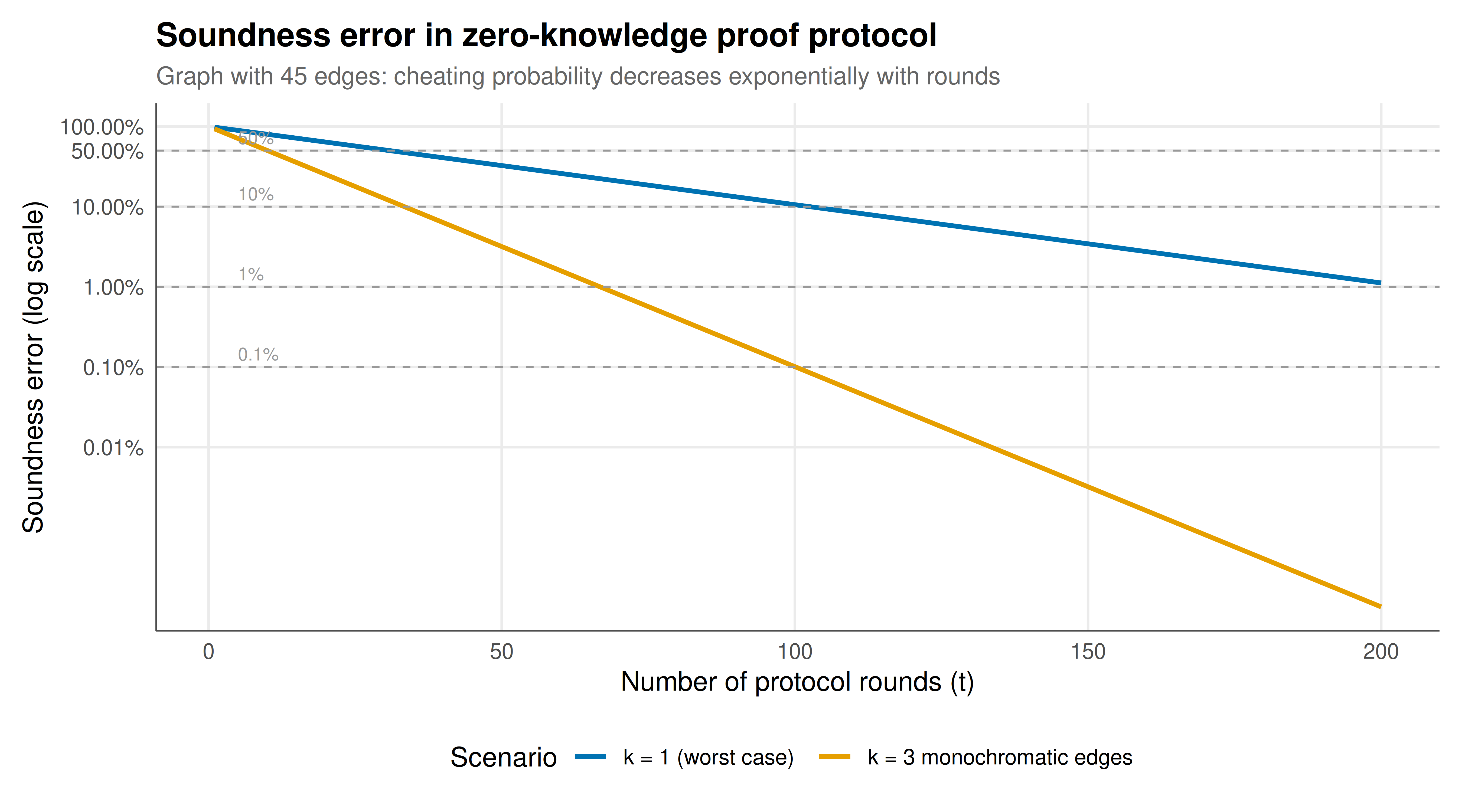
#| fig-cap: "Soundness error probability as a function of protocol rounds for a zero-knowledge proof of graph three-colourability. The worst case (k equals 1 monochromatic edge) is shown alongside the scenario with three monochromatic edges. Horizontal dashed lines mark common security targets. The exponential decay ensures practical security within a manageable number of rounds. Rendered using the Okabe-Ito palette."
#| dev: [png, pdf]
#| dpi: 300
#| fig-width: 9
#| fig-height: 5
target_df <- data.frame(
  label = c("50%", "10%", "1%", "0.1%"),
  y = c(0.5, 0.1, 0.01, 0.001)
)

p_static <- ggplot(results_df, aes(x = rounds, y = error,
                                    color = scenario_label)) +
  geom_line(linewidth = 1.0) +
  geom_hline(data = target_df, aes(yintercept = y),
             linetype = "dashed", color = okabe_ito[8], linewidth = 0.4) +
  geom_text(data = target_df, aes(x = 5, y = y, label = label),
            inherit.aes = FALSE, vjust = -0.5, hjust = 0,
            size = 2.8, color = okabe_ito[8]) +
  scale_y_log10(labels = scales::label_percent(accuracy = 0.01),
                breaks = c(1, 0.5, 0.1, 0.01, 0.001, 0.0001)) +
  scale_color_manual(values = okabe_ito[c(5, 1)]) +
  labs(title = "Soundness error in zero-knowledge proof protocol",
       subtitle = sprintf("Graph with %d edges: cheating probability decreases exponentially with rounds", m_edges),
       x = "Number of protocol rounds (t)",
       y = "Soundness error (log scale)",
       color = "Scenario") +
  theme_publication() +
  theme(legend.position = "bottom")

print(p_static)
```
## Interactive figure
```{r}
#| label: fig-zkp-interactive
#| fig-cap: "Interactive visualization of soundness error decay. Hover to see the exact number of rounds, soundness error, and the corresponding security level for each scenario."
p_int <- ggplot(results_df, aes(x = rounds, y = error,
    color = scenario_label,
    text = sprintf("Rounds: %d\nSoundness error: %.6f\nSecurity: %.2f bits\nScenario: %s",
                   rounds, error, -log2(error), scenario_label))) +
  geom_line(linewidth = 0.7) +
  scale_y_log10(labels = scales::label_percent()) +
  scale_color_manual(values = okabe_ito[c(5, 1)]) +
  labs(title = "Soundness error decay",
       x = "Protocol rounds", y = "Soundness error (log scale)",
       color = "Scenario") +
  theme_publication()

ggplotly(p_int, tooltip = "text") |>
  config(displaylogo = FALSE,
         modeBarButtonsToRemove = c("select2d", "lasso2d"))
```
## Interpretation
The computational results and visualizations illuminate several key aspects of zero-knowledge proofs as strategic games, providing insights that bridge cryptographic security analysis and game-theoretic reasoning. The exponential decay of the soundness error is the most visually striking feature, and it carries deep implications for protocol design and strategic behaviour.
The most immediate observation is that the soundness error decreases exponentially with the number of rounds, which means that practical security is achievable within a feasible number of rounds even for large graphs. For a graph with 45 edges, achieving a soundness error below 1% requires approximately 207 rounds in the worst case. While this may seem computationally expensive, each round involves only a commitment to vertex colours and the revelation of two colours -- operations that are extremely fast with modern cryptographic primitives. The key insight is that exponential decay is qualitatively different from linear or polynomial decay: doubling the number of rounds squares the security level rather than merely doubling it. This is why interactive proofs are practical despite requiring multiple rounds of communication.
The comparison between the worst case (one monochromatic edge) and the three-edge case reveals an important strategic dimension. A cheating prover who presents a colouring with more monochromatic edges is detected faster, so the optimal cheating strategy minimizes the number of monochromatic edges. This means the prover faces an optimization problem: how to construct a "near-valid" colouring that minimizes detection probability. In game-theoretic terms, the cheater's optimal strategy is to play the worst case (exactly one monochromatic edge), which maximizes the expected number of rounds survived. This adversarial optimization is precisely the type of analysis that security proofs must consider, and it maps directly to the minimax framework in game theory.
The simulation results confirm the theoretical analysis with high precision. Out of 10,000 simulated cheaters attempting 150 rounds, the fraction that passes all rounds closely matches the theoretical prediction. This validates the independence assumption that underlies the protocol: because the prover re-randomizes the colouring in each round, the detection events across rounds are indeed independent. In a game-theoretic context, this re-randomization is a commitment device that prevents the verifier from correlating queries across rounds. Without re-randomization, a sophisticated verifier could adaptively choose edges based on previous responses, potentially extracting information about the colouring -- violating the zero-knowledge property.
The connection to mechanism design becomes clear when we consider the protocol designer's problem. The designer must choose the number of rounds (the mechanism parameter) to balance two objectives: convincing the verifier that the prover's claim is genuine (soundness) while preventing the verifier from learning the actual colouring (zero-knowledge). Increasing the number of rounds improves soundness but increases the computational cost and the amount of interaction. The optimal number of rounds depends on the application's security requirements and the cost of communication. This is a classic mechanism design trade-off, where the designer optimizes over the space of protocols rather than over the space of allocations.
The strategic verification perspective also sheds light on the role of computational assumptions in cryptography. In our analysis, we assumed that the commitment scheme is perfectly hiding (the verifier learns nothing from the commitments alone) and perfectly binding (the prover cannot change committed values). In practice, these properties are achieved only computationally -- they hold against computationally bounded adversaries. This introduces a bounded rationality element into the game: the prover and verifier are not fully rational in the game-theoretic sense but are constrained by computational feasibility. This connection between computational complexity and strategic rationality is a frontier area of research that promises to deepen our understanding of both fields.
## Extensions and related tutorials
- [Commitment schemes and strategic play](../commitment-schemes-game-theory/index.qmd) -- how cryptographic commitments enable strategic advantages in games.
- Mechanism design with verification (tutorial not yet available) -- designing mechanisms where agents' claims can be partially verified.
- [Bayesian games and incomplete information](../../bayesian-methods/bayesian-games-incomplete-information/) -- formal treatment of games with private information, the foundation of prover-verifier interactions.
- [Repeated games and monitoring](../../foundations/folk-theorem-perfect-monitoring/index.qmd) -- strategic inspection games that share structural similarities with zero-knowledge protocols.
## References
::: {#refs}
:::