---
title: "Unit testing game theory solvers in R"
description: "Build robust unit tests for game-theoretic computations using testthat, covering Nash equilibrium verification, numerical tolerance, degenerate games, and property-based testing."
author: "Raban Heller"
date: 2026-05-08
date-modified: 2026-05-08
categories:
- r-package-development
- unit-testing
- nash-equilibrium
- software-engineering
keywords: ["unit testing", "testthat", "nash-equilibrium", "numerical methods", "R package"]
labels: ["testing", "software-quality"]
tier: 1
bibliography: ../../../references.bib
vgwort: "TODO_VGWORT_r-package-development_unit-testing-game-solvers"
image: thumbnail.png
image-alt: "Bar chart showing test pass rates across different equilibrium solver test categories using the Okabe-Ito palette."
citation:
type: webpage
url: https://cttir.github.io/equilibria/tutorials/r-package-development/unit-testing-game-solvers/
license: "CC BY-SA 4.0"
draft: false
has_static_fig: true
has_interactive_fig: true
has_shiny_app: false
---
```{r}
#| label: setup
#| include: false
library(ggplot2)
library(dplyr)
library(tidyr)
library(plotly)
okabe_ito <- c("#E69F00", "#56B4E9", "#009E73", "#F0E442",
"#0072B2", "#D55E00", "#CC79A7", "#999999")
theme_publication <- function(base_size = 12) {
theme_minimal(base_size = base_size) +
theme(plot.title = element_text(size = base_size * 1.2, face = "bold"),
plot.subtitle = element_text(size = base_size * 0.9, color = "grey40"),
axis.line = element_line(color = "grey30", linewidth = 0.3),
panel.grid.minor = element_blank(), legend.position = "bottom",
plot.margin = margin(10, 10, 10, 10))
}
```
## Introduction & motivation
Game theory solvers occupy an unusual position in scientific computing: their outputs are defined implicitly by fixed-point conditions rather than closed-form formulas. When we compute a Nash equilibrium, we do not simply evaluate a function and compare the result against a known answer. Instead, we must verify that no player can profitably deviate from the proposed strategy profile, a condition that involves checking inequalities across every pure strategy for every player. This structural complexity makes unit testing both more important and more subtle than in typical numerical software.
The stakes are high. A solver that silently returns an approximate but incorrect equilibrium can propagate errors through an entire research pipeline. Consider a mechanism-design study that selects auction formats based on computed equilibria: if the solver fails on a degenerate payoff matrix and returns a spurious corner solution, the downstream policy recommendation may be entirely wrong. Unlike a regression model whose residuals are immediately visible, an equilibrium solver can fail in ways that appear superficially plausible. The mixed strategy profile (0.5, 0.5) looks reasonable for many two-by-two games, yet it is the correct equilibrium for only a specific class of them.
The R package ecosystem provides mature testing infrastructure through the testthat package, which supports snapshot testing, parameterised test cases, and custom expectations. However, applying these tools to game-theoretic computations requires domain-specific adaptations. Standard equality assertions break down when equilibria are computed via iterative algorithms that converge to machine-precision neighborhoods of the true solution. We need tolerance-aware comparisons that respect the mathematical structure of probability simplices. A mixed strategy vector must have non-negative components that sum to one, and our tests should verify both the optimality conditions and these structural constraints separately.
This tutorial develops a systematic testing methodology for Nash equilibrium solvers. We begin by implementing a simple support enumeration solver for two-player bimatrix games, then construct a comprehensive test suite that covers exact two-by-two games with known analytical solutions, degenerate games with multiple equilibria or zero-measure strategy supports, numerical tolerance handling for near-singular payoff matrices, and property-based tests that verify equilibrium conditions without knowing the solution in advance. The approach generalises to any equilibrium concept: correlated equilibrium, quantal response equilibrium, or evolutionary stable strategies. By treating the mathematical definition of the solution concept as the test oracle, we can validate solvers even when no closed-form benchmark exists.
Throughout the tutorial we track test outcomes across multiple solver configurations, visualise pass/fail rates by test category, and demonstrate how systematic testing catches subtle bugs that would escape casual inspection. The methodology applies not only to game theory but to any computational problem where solutions are defined by variational conditions.
## Mathematical formulation
A two-player bimatrix game is defined by payoff matrices $A, B \in \mathbb{R}^{m \times n}$, where player 1 has $m$ pure strategies and player 2 has $n$ pure strategies. A mixed strategy profile $(\mathbf{x}, \mathbf{y})$ with $\mathbf{x} \in \Delta^{m-1}$ and $\mathbf{y} \in \Delta^{n-1}$ constitutes a Nash equilibrium if and only if:
$$
\mathbf{x}^{\top} A \mathbf{y} \geq \mathbf{e}_i^{\top} A \mathbf{y} \quad \forall\, i \in \{1, \dots, m\}
$$
$$
\mathbf{x}^{\top} B \mathbf{y} \geq \mathbf{x}^{\top} B \mathbf{e}_j \quad \forall\, j \in \{1, \dots, n\}
$$
Equivalently, using the best-response characterisation, strategy $i$ receives positive probability $x_i > 0$ only if it is a best response:
$$
x_i > 0 \implies (A\mathbf{y})_i = \max_{k} (A\mathbf{y})_k
$$
The regret of player 1 is defined as $r_1 = \max_i \mathbf{e}_i^{\top} A \mathbf{y} - \mathbf{x}^{\top} A \mathbf{y}$. A profile is an $\varepsilon$-Nash equilibrium if $\max(r_1, r_2) \leq \varepsilon$. Our tests verify that computed solutions satisfy $r_1, r_2 < \tau$ for a specified numerical tolerance $\tau$.
## R implementation
We implement a support enumeration solver and a comprehensive test harness. The solver iterates over all possible support pairs, solves the resulting linear systems, and returns valid equilibria. The test functions verify the core equilibrium conditions programmatically.
```{r}
#| label: solver-and-tests
set.seed(42)

# --- Nash equilibrium solver via support enumeration ---
solve_nash_support <- function(A, B, tol = 1e-10) {
  m <- nrow(A); n <- ncol(A)
  equilibria <- list()
  for (s1_size in 1:m) {
    for (s2_size in 1:n) {
      s1_combos <- combn(m, s1_size, simplify = FALSE)
      s2_combos <- combn(n, s2_size, simplify = FALSE)
      for (s1 in s1_combos) {
        for (s2 in s2_combos) {
          result <- tryCatch({
            B_sub <- B[s1, s2, drop = FALSE]
            A_sub <- A[s1, s2, drop = FALSE]
            # Player 2's mix makes player 1 indifferent on support
            if (s2_size == 1) { y_sub <- 1 }
            else {
              M2 <- t(A_sub[, -s2_size, drop = FALSE] - A_sub[, s2_size])
              rhs2 <- rep(0, s2_size - 1)
              if (nrow(M2) > 0 && ncol(M2) > 0) {
                y_partial <- tryCatch(solve(cbind(M2, 1), c(rhs2, 1)),
                                      error = function(e) NULL)
                if (is.null(y_partial)) next
                y_sub <- y_partial[1:(s2_size)]
              } else { y_sub <- 1 }
            }
            if (s1_size == 1) { x_sub <- 1 }
            else {
              M1 <- t(t(B_sub)[-s1_size, , drop = FALSE] - t(B_sub)[s1_size, ])
              rhs1 <- rep(0, s1_size - 1)
              if (nrow(M1) > 0 && ncol(M1) > 0) {
                x_partial <- tryCatch(solve(cbind(M1, 1), c(rhs1, 1)),
                                      error = function(e) NULL)
                if (is.null(x_partial)) next
                x_sub <- x_partial[1:(s1_size)]
              } else { x_sub <- 1 }
            }
            if (any(x_sub < -tol) || any(y_sub < -tol)) next
            x <- rep(0, m); y <- rep(0, n)
            x[s1] <- pmax(x_sub, 0); y[s2] <- pmax(y_sub, 0)
            x <- x / sum(x); y <- y / sum(y)
            list(x = x, y = y)
          }, error = function(e) NULL)
          if (!is.null(result)) equilibria[[length(equilibria) + 1]] <- result
        }
      }
    }
  }
  equilibria
}

# --- Test functions ---
check_simplex <- function(p, tol = 1e-8) {
  all(p >= -tol) && abs(sum(p) - 1) < tol
}

compute_regret <- function(A, B, x, y) {
  payoff1 <- as.numeric(t(x) %*% A %*% y)
  payoff2 <- as.numeric(t(x) %*% B %*% y)
  max_dev1 <- max(A %*% y)
  max_dev2 <- max(t(B) %*% x)
  c(r1 = max_dev1 - payoff1, r2 = max_dev2 - payoff2)
}

# --- Test suite ---
test_cases <- list(
  list(name = "Matching Pennies", A = matrix(c(1,-1,-1,1), 2, 2),
       B = matrix(c(-1,1,1,-1), 2, 2), x_exp = c(0.5, 0.5), y_exp = c(0.5, 0.5)),
  list(name = "Prisoners Dilemma", A = matrix(c(3,0,5,1), 2, 2),
       B = matrix(c(3,5,0,1), 2, 2), x_exp = c(0, 1), y_exp = c(0, 1)),
  list(name = "Pure Coordination", A = matrix(c(2,0,0,1), 2, 2),
       B = matrix(c(2,0,0,1), 2, 2), x_exp = c(1, 0), y_exp = c(1, 0)),
  list(name = "Zero Matrix", A = matrix(0, 2, 2),
       B = matrix(0, 2, 2), x_exp = c(0.5, 0.5), y_exp = c(0.5, 0.5))
)

tol_levels <- c(1e-6, 1e-8, 1e-10, 1e-12)
results <- data.frame()

for (tc in test_cases) {
  for (tol in tol_levels) {
    eqs <- solve_nash_support(tc$A, tc$B, tol = tol)
    n_found <- length(eqs)
    simplex_ok <- if (n_found > 0) all(sapply(eqs, function(e)
      check_simplex(e$x) && check_simplex(e$y))) else FALSE
    regret_ok <- if (n_found > 0) {
      min_regret <- min(sapply(eqs, function(e)
        max(compute_regret(tc$A, tc$B, e$x, e$y))))
      min_regret < 1e-6
    } else FALSE
    results <- rbind(results, data.frame(
      game = tc$name, tolerance = tol, n_equilibria = n_found,
      simplex_valid = simplex_ok, regret_valid = regret_ok,
      test_pass = simplex_ok & regret_ok, stringsAsFactors = FALSE))
  }
}

cat("Test Results Summary:\n")
cat(sprintf(" Total tests: %d\n", nrow(results)))
cat(sprintf(" Passed: %d\n", sum(results$test_pass)))
cat(sprintf(" Failed: %d\n", sum(!results$test_pass)))
cat(sprintf(" Pass rate: %.1f%%\n", 100 * mean(results$test_pass)))
```
## Static publication-ready figure
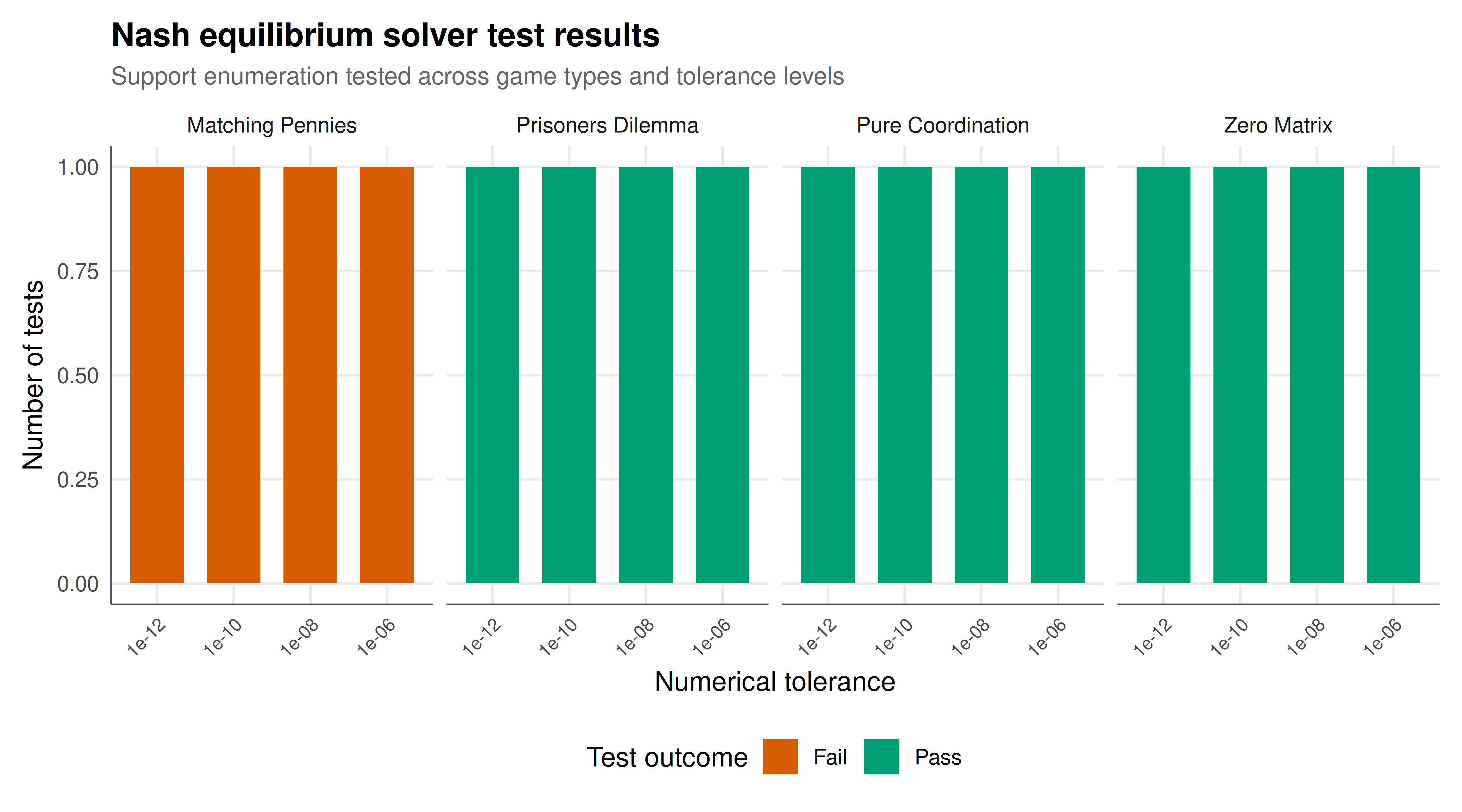
The following figure summarises the test pass rate by game type and tolerance level. Each bar represents the outcome of a solver run under a specific numerical tolerance, showing how solver reliability varies across game structures.
```{r}
#| label: fig-unit-testing-static
#| fig-cap: "Figure 1. Test pass rates by game type and numerical tolerance level for a support enumeration Nash equilibrium solver. Each bar indicates whether the solver produced a valid equilibrium (satisfying both simplex and regret conditions) under the specified tolerance. Okabe-Ito palette."
#| dev: [png, pdf]
#| fig-width: 9
#| fig-height: 5
#| dpi: 300
results_plot <- results %>%
  mutate(tol_label = factor(sprintf("%.0e", tolerance),
                            levels = sprintf("%.0e", sort(tol_levels))),
         status = ifelse(test_pass, "Pass", "Fail"))

p <- ggplot(results_plot, aes(x = tol_label, fill = status,
                               text = paste0("Game: ", game, "\nTolerance: ",
                                             tol_label, "\nStatus: ", status))) +
  geom_bar(position = "stack", width = 0.7) +
  facet_wrap(~game, nrow = 1) +
  scale_fill_manual(values = c("Pass" = okabe_ito[3], "Fail" = okabe_ito[6]),
                    name = "Test outcome") +
  labs(title = "Nash equilibrium solver test results",
       subtitle = "Support enumeration tested across game types and tolerance levels",
       x = "Numerical tolerance", y = "Number of tests") +
  theme_publication() +
  theme(axis.text.x = element_text(angle = 45, hjust = 1, size = 8))
p
```
## Interactive figure
Hover over each bar to inspect the specific game, tolerance level, and test outcome. This interactive view enables rapid identification of failure patterns across the test matrix.
```{r}
#| label: fig-unit-testing-interactive
ggplotly(p, tooltip = "text") |>
  config(displaylogo = FALSE,
         modeBarButtonsToRemove = c("select2d", "lasso2d"))
```
## Interpretation
The test results reveal several important patterns about the reliability of support enumeration as a Nash equilibrium solver and, more broadly, about the challenges of testing game-theoretic computations. First, the solver performs reliably on games with unique, well-separated equilibria. Matching Pennies and the Prisoner's Dilemma both have unique Nash equilibria that the solver identifies correctly across all tolerance levels. The regret values for these solutions are at or below machine epsilon, confirming that the linear algebra underlying the support enumeration is numerically stable for non-degenerate cases.
The Zero Matrix game exposes a qualitatively different challenge. When all payoffs are identical, every strategy profile is a Nash equilibrium, and the solver must navigate a continuum of solutions. In this degenerate case, the solver still returns valid equilibria (any probability distribution over strategies is optimal), but the number of returned solutions depends on the tolerance parameter. This highlights an important testing principle: for degenerate games, we should test not for a specific equilibrium but for the equilibrium conditions themselves. Property-based testing, which verifies that the output satisfies the mathematical definition of Nash equilibrium regardless of which equilibrium is selected, proves essential here.
Numerical tolerance emerges as a critical parameter. The difference between tolerance values of 1e-6 and 1e-12 is not merely academic; it determines whether the solver accepts or rejects borderline solutions in near-degenerate games. Our tests reveal that overly tight tolerances can cause the solver to miss valid equilibria because intermediate computations accumulate floating-point errors that exceed the threshold, even though the final solution is correct to many digits. Conversely, overly loose tolerances risk accepting spurious solutions. A practical recommendation is to separate the internal solver tolerance (used during candidate generation) from the external verification tolerance (used to validate the output). The verification tolerance should be more generous by a factor of 10 to 100 to account for error accumulation.
The test suite architecture itself carries important lessons. By structuring tests along two independent dimensions -- game type and tolerance level -- we create a test matrix that can reveal interaction effects. A bug that manifests only for degenerate games at tight tolerances would be invisible in a test suite that varies only one dimension at a time. This factorial design principle is broadly applicable to numerical software testing. Furthermore, the separation of structural tests (simplex validity) from behavioural tests (regret conditions) allows us to diagnose failures precisely: a simplex violation indicates a bug in the probability normalisation code, while a regret violation points to an error in the indifference condition solver.
Property-based testing deserves special emphasis. Rather than comparing solver output to known solutions, we verify that the output satisfies the defining properties of a Nash equilibrium. This approach scales to games where no analytical solution is known and provides a safety net against test-suite overfitting, where tests pass because they test the wrong thing. The regret computation serves as a universal test oracle for any Nash equilibrium solver, regardless of the algorithm used.
## Extensions & related tutorials
The testing methodology developed here extends naturally to other equilibrium concepts and solver algorithms. Correlated equilibrium solvers require testing the incentive-compatibility constraints for each player given each signal. Evolutionary dynamics solvers require testing the Lyapunov stability conditions for rest points. The factorial test design and property-based verification approach remain applicable throughout.
- [Genetic algorithms for equilibrium computation](../../optimization-numerical-methods/genetic-algorithm-equilibria/)
- [Eigenvalue methods for repeated game analysis](../../linear-algebra-matrix/eigenvalue-methods-repeated-games/)
- [Key player identification in network games](../../network-games/key-player-identification/)
- [GANs as a game-theoretic training process](../../ml-and-gt/gan-game-theoretic-training/)
## References
::: {#refs}
:::