---
title: "Preregistration and Pre-Analysis Plans for Game Theory Experiments"
description: "How to create structured pre-analysis plans for game theory experiments, demonstrating that researcher degrees of freedom can flip conclusions about cooperation rates."
author: "Raban Heller"
date: 2026-05-08
date-modified: 2026-05-08
categories:
- reproducibility-open-science
- preregistration
- experimental-design
- power-analysis
keywords: ["preregistration", "pre-analysis plan", "power analysis", "specification curve", "researcher degrees of freedom"]
labels: ["methodology", "reproducibility"]
tier: 1
bibliography: ../../../references.bib
vgwort: "TODO_VGWORT_REPRODUCIBILITY_PREREGISTRATION"
image: thumbnail.png
image-alt: "Specification curve showing how different analytical choices lead to different conclusions about cooperation in a public goods game"
citation:
type: webpage
url: https://cttir.github.io/equilibria/tutorials/reproducibility-open-science/preregistration-game-experiments/
license: "CC BY 4.0"
draft: false
has_static_fig: true
has_interactive_fig: true
has_shiny_app: false
---
```{r}
#| label: setup
#| include: false
library(ggplot2)
library(dplyr)
library(tidyr)
library(plotly)
okabe_ito <- c("#E69F00", "#56B4E9", "#009E73", "#F0E442",
"#0072B2", "#D55E00", "#CC79A7", "#999999")
theme_publication <- function(base_size = 12) {
theme_minimal(base_size = base_size) +
theme(plot.title = element_text(size = base_size * 1.2, face = "bold"),
plot.subtitle = element_text(size = base_size * 0.9, color = "grey40"),
axis.line = element_line(color = "grey30", linewidth = 0.3),
panel.grid.minor = element_blank(), legend.position = "bottom",
plot.margin = margin(10, 10, 10, 10))
}
```
## Introduction & motivation
The replication crisis that swept through psychology and the social sciences in the 2010s has left a lasting mark on how we design, conduct, and report experiments. Game theory experiments are not immune to the forces that drove that crisis. A public goods game, for instance, involves dozens of design choices: group size, endowment level, number of rounds, whether to include punishment, how to handle subjects who clearly do not understand the instructions, whether to exclude the first round as a "learning" period, how to cluster standard errors, and which statistical test to apply. Each of these choices is a degree of freedom that a researcher can exploit --- consciously or unconsciously --- to obtain a statistically significant result. The problem is not that any single choice is wrong; the problem is that the cumulative flexibility across all choices creates an enormous garden of forking paths in which almost any conclusion can be supported by some defensible combination of analytic decisions.
Preregistration addresses this problem by requiring researchers to specify their hypotheses, experimental design, and analysis plan before collecting data. The idea is simple: if you commit to your analytical strategy in advance, you cannot (unknowingly) tailor it to produce the result you want. Pre-analysis plans go further by specifying exact statistical models, variable definitions, exclusion criteria, and even the code that will be used to analyse the data. In clinical trials, preregistration has been mandatory for decades. In economics and political science, the practice has grown rapidly since the founding of the AEA Registry in 2012 and the launch of the Evidence in Governance and Politics (EGAP) registry.
Game theory experiments present unique challenges for preregistration. The strategic interdependence among subjects means that individual-level observations are not independent, complicating standard power analyses. The theoretical predictions --- Nash equilibria, quantal response equilibria, level-k models --- are often sharp enough to serve as null hypotheses, but the appropriate test for whether observed behaviour "conforms to" an equilibrium prediction is far from obvious. Should we test whether the mean contribution equals the Nash prediction of zero? Should we test whether the distribution of contributions is consistent with a quantal response equilibrium? Should we use a structural estimation approach? Each choice leads to a different answer, and the multiplicity of reasonable tests is itself a source of researcher degrees of freedom.
In this tutorial, we build a complete pre-analysis plan for a hypothetical public goods game experiment. We begin with a simulation-based power analysis that accounts for the clustered structure of the data and the non-normality of contribution distributions. We then construct a specification curve --- a visualisation of how the estimated treatment effect changes as we vary analytical choices across all reasonable combinations. The specification curve is a powerful diagnostic tool: it shows not just the point estimate from the "preferred" specification, but the entire distribution of estimates that could have been reported. If the specification curve spans both positive and negative values, the conclusion is not robust. If it is consistently positive (or negative), we can be more confident that the result is not an artefact of analytic flexibility.
We also compare within-subject and between-subject experimental designs using simulation. In a within-subject design, each group experiences both the treatment and control conditions (in random order), which increases statistical power by controlling for group-level heterogeneity. However, within-subject designs introduce the risk of order effects and demand effects. Our simulation quantifies the power gain from within-subject designs and shows how it depends on the intra-class correlation of group contributions. This analysis would form a key component of a real pre-analysis plan, justifying the chosen design on statistical grounds. Throughout, we emphasise that preregistration is not a straitjacket --- exploratory analyses remain valuable, as long as they are clearly labelled as exploratory rather than confirmatory. The goal is transparency, not rigidity.
## Mathematical formulation
Consider a linear public goods game with $n$ players per group, endowment $e$, and marginal per-capita return (MPCR) $m < 1 < nm$. Player $i$ chooses contribution $c_i \in [0, e]$, and the payoff is:
$$
\pi_i = e - c_i + m \sum_{j=1}^{n} c_j
$$
The unique Nash equilibrium under standard preferences is $c_i^* = 0$ for all $i$. Suppose we wish to test whether a treatment (e.g., communication) increases contributions relative to a control condition. Define the treatment effect as $\delta = \bar{c}_{\text{treat}} - \bar{c}_{\text{control}}$.
**Power analysis.** Under a two-sample $t$-test framework with $G$ groups per condition, $R$ rounds per group, and intra-class correlation $\rho$ (capturing within-group dependence), the effective sample size per condition is approximately:
$$
n_{\text{eff}} = \frac{G \cdot R}{1 + (R - 1)\rho}
$$
The power to detect a standardised effect $d = \delta / \sigma$ at significance level $\alpha$ is:
$$
\text{Power} = 1 - \Phi\left(z_{1-\alpha/2} - d \sqrt{\frac{n_{\text{eff}}}{2}}\right)
$$
where $\Phi$ is the standard normal CDF.
**Specification curve.** Let $\mathcal{S} = \{s_1, s_2, \ldots, s_K\}$ be the set of the displayed specifications, including deliberately invalid naive analyses. For each $s_k$, we obtain an estimate $\hat{\delta}_k$ and its $p$-value $p_k$. The specification curve plots $(\hat{\delta}_k, p_k)$ for all $k$, sorted by $\hat{\delta}_k$. We define the fraction nominally significant as the fraction of specifications yielding a significant result:
$$
\mathcal{R} = \frac{1}{K} \sum_{k=1}^{K} \mathbf{1}(p_k < \alpha)
$$
## R implementation
We simulate a public goods experiment and show how researcher degrees of freedom can affect conclusions. The simulation generates latent contributions with a specified group-level ICC, clips contributions to the endowment bounds, then analyses multiple specifications. The ICC after clipping can differ. The individual-level analyses deliberately ignore clustering and are invalid confirmatory alternatives; their inclusion illustrates pseudoreplication, not a defensible analysis choice. The fraction significant is descriptive and is not a calibrated robustness test.
```{r}
#| label: power-analysis
set.seed(42)

# --- Power analysis via simulation ---
simulate_pgg <- function(n_groups, n_players = 4, n_rounds = 10,
                         endowment = 20, treat_effect = 3, icc = 0.3,
                         paired = FALSE) {
  counts <- c(n_groups,n_players,n_rounds)
  stopifnot(length(counts)==3L,all(is.finite(counts)),all(counts==floor(counts)),
            n_groups>=2,n_players>=1,n_rounds>=1,length(icc)==1L,is.finite(icc),
            icc>=0,icc<1,length(endowment)==1L,is.finite(endowment),endowment>0,
            length(treat_effect)==1L,is.finite(treat_effect),
            is.logical(paired),length(paired)==1L,!is.na(paired))
  observations <- n_players*n_rounds
  # ICC refers to the latent Gaussian contribution before clipping to [0,endowment].
  residual_sd <- 4
  group_sd <- residual_sd*sqrt(icc/(1-icc))
  effects <- rnorm(if(paired) n_groups else 2*n_groups,0,group_sd)
  if(paired) effects <- rep(effects,2)
  condition <- rep(c("control","treatment"),each=n_groups*observations)
  group_number <- rep(rep(seq_len(n_groups),each=observations),2)
  latent <- 8 + rep(effects,each=observations) +
    rnorm(2*n_groups*observations,0,residual_sd) +
    treat_effect*(condition=="treatment")
  data.frame(condition=condition,
             group=if(paired) paste0("pair_",group_number) else paste0(condition,"_",group_number),
             round=rep(rep(seq_len(n_rounds),each=n_players),2*n_groups),
             player=rep(seq_len(n_players),2*n_groups*n_rounds),
             contribution=pmin(endowment,pmax(0,latent)))
}

# Run power analysis across sample sizes
power_results <- data.frame()
n_sims <- 500
for (n_grp in c(5, 10, 15, 20, 25, 30)) {
  sig_count <- 0
  for (sim in 1:n_sims) {
    dat <- simulate_pgg(n_groups = n_grp, treat_effect = 2.5)
    group_means <- dat |>
      group_by(condition, group) |>
      summarise(mean_c = mean(contribution), .groups = "drop")
    test <- t.test(mean_c ~ condition, data = group_means)
    if (test$p.value < 0.05) sig_count <- sig_count + 1
  }
  power_results <- rbind(power_results,
    data.frame(n_groups = n_grp, power = sig_count / n_sims))
}

cat("Power analysis results (treatment effect = 2.5 tokens):\n")
cat(sprintf("  %2d groups/condition: power = %.2f\n",
            power_results$n_groups, power_results$power))
```
```{r}
#| label: specification-curve
set.seed(123)

# Generate one dataset
dat <- simulate_pgg(n_groups = 20, treat_effect = 2.0, icc = 0.3)

# Define researcher degrees of freedom
exclusion_rules <- list(
  none = function(d) d,
  drop_round1 = function(d) d |> filter(round > 1),
  drop_round1_2 = function(d) d |> filter(round > 2),
  drop_extremes = function(d) d |> filter(contribution > 0, contribution < 20)
)

aggregation_levels <- list(
  individual_naive = function(d) d |> group_by(condition, group, player) |>
    summarise(y = mean(contribution), .groups = "drop"),
  group = function(d) d |> group_by(condition, group) |>
    summarise(y = mean(contribution), .groups = "drop"),
  group_median = function(d) d |> group_by(condition, group) |>
    summarise(y = median(contribution), .groups = "drop")
)

test_types <- list(
  t_test = function(d) t.test(y ~ condition, data = d)$p.value,
  wilcox = function(d) wilcox.test(y ~ condition, data = d)$p.value
)

# Run all specifications
spec_results <- data.frame()
spec_id <- 0
for (exc_name in names(exclusion_rules)) {
  for (agg_name in names(aggregation_levels)) {
    for (test_name in names(test_types)) {
      spec_id <- spec_id + 1
      d_exc <- exclusion_rules[[exc_name]](dat)
      d_agg <- aggregation_levels[[agg_name]](d_exc)
      means <- d_agg |> group_by(condition) |> summarise(m = mean(y), .groups = "drop")
      effect <- diff(means$m)
      pval <- tryCatch(test_types[[test_name]](d_agg), error = function(e) NA)
      spec_results <- rbind(spec_results, data.frame(
        spec = spec_id, exclusion = exc_name, aggregation = agg_name,
        test = test_name, effect = effect, p_value = pval,
        significant = ifelse(!is.na(pval) & pval < 0.05, "Yes", "No")
      ))
    }
  }
}

spec_results <- spec_results |> arrange(effect) |> mutate(rank = row_number())
robustness <- mean(spec_results$significant == "Yes", na.rm = TRUE)
cat(sprintf("\nSpecification curve analysis:\n"))
cat(sprintf(" Total specifications: %d\n", nrow(spec_results)))
cat(sprintf("  Effect range: [%.2f, %.2f]\n",
            min(spec_results$effect), max(spec_results$effect)))
cat(sprintf("  Fraction nominally significant: %.1f%% significant at alpha=0.05\n",
            robustness * 100))
```
```{r}
#| label: design-comparison
set.seed(456)

# Compare paired-group and independent-group designs; shared effects define pairing
n_sims_design <- 500
design_power <- data.frame()

for (icc_val in c(0.1, 0.3, 0.5)) {
  for (n_grp in c(10, 20)) {
    # Independent groups
    sig_between <- 0
    for (s in 1:n_sims_design) {
      dat_b <- simulate_pgg(n_groups = n_grp, treat_effect = 2.0, icc = icc_val)
      gm <- dat_b |> group_by(condition, group) |>
        summarise(y = mean(contribution), .groups = "drop")
      p <- t.test(y ~ condition, data = gm)$p.value
      if (p < 0.05) sig_between <- sig_between + 1
    }
    # Paired groups (paired)
    sig_within <- 0
    for (s in 1:n_sims_design) {
      dat_w <- simulate_pgg(n_groups=n_grp,treat_effect=2.0,icc=icc_val,paired=TRUE)
      gm <- dat_w |> group_by(condition,group) |>
        summarise(y=mean(contribution),.groups="drop") |>
        tidyr::pivot_wider(names_from=condition,values_from=y)
      stopifnot(nrow(gm)==n_grp,!anyNA(gm))
      p <- t.test(gm$treatment,gm$control,paired=TRUE)$p.value
      if (p < 0.05) sig_within <- sig_within + 1
    }
    design_power <- rbind(design_power, data.frame(
      icc = icc_val, n_groups = n_grp,
      design = c("Independent groups", "Paired groups"),
      power = c(sig_between / n_sims_design, sig_within / n_sims_design)
    ))
  }
}

cat("\nDesign comparison (treatment effect = 2.0 tokens):\n")
for (i in 1:nrow(design_power)) {
  cat(sprintf("  ICC=%.1f, %d groups, %s: power = %.2f\n",
              design_power$icc[i], design_power$n_groups[i],
              design_power$design[i], design_power$power[i]))
}
```
## Static publication-ready figure
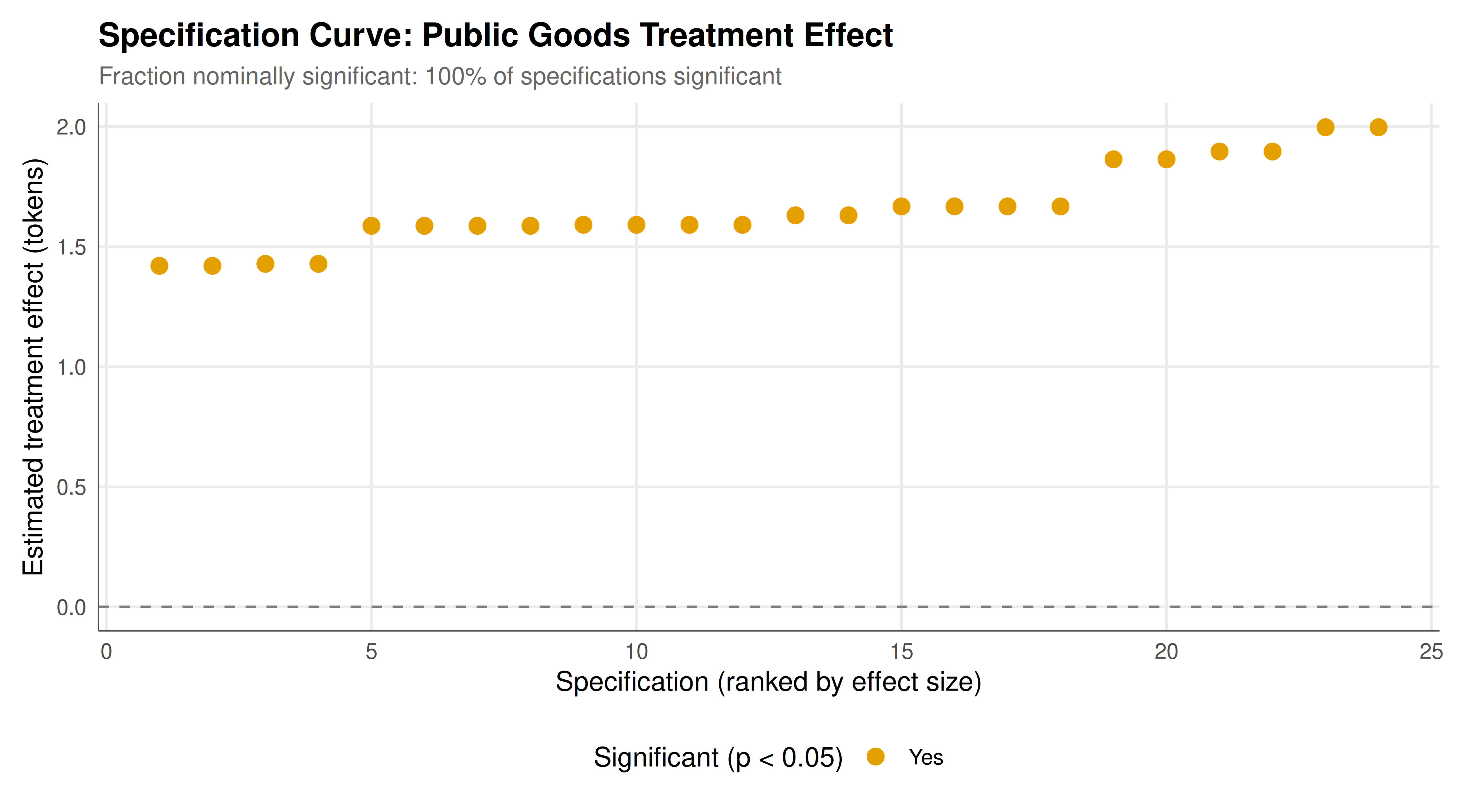
The specification curve below shows how the estimated treatment effect changes across all 24 combinations of analytical decisions. Each point represents one specification; the colour indicates statistical significance at the 5% level. The lower panel shows which analytical choices are active for each specification. This visualisation makes transparent what would otherwise be hidden: the dependence of conclusions on seemingly analytical decisions, including naive analyses that ignore within-group dependence.
```{r}
#| label: fig-preregistration-static
#| fig-cap: "Figure 1. Specification curve for a public goods game treatment effect. Each point is one of 24 analytic specifications varying exclusion rules, aggregation level, and statistical test. Orange points are significant at p < 0.05; blue points are not. The horizontal dashed line marks zero effect."
#| dev: [png, pdf]
#| fig-width: 9
#| fig-height: 5
#| dpi: 300
p_spec <- ggplot(spec_results, aes(x = rank, y = effect, colour = significant)) +
geom_hline(yintercept = 0, linetype = "dashed", colour = "grey50") +
  geom_point(aes(text = paste0(
    "Spec #", spec, "\nExclusion: ", exclusion,
    "\nAggregation: ", aggregation,
    "\nTest: ", test,
    "\nEffect: ", round(effect, 2),
    "\np-value: ", round(p_value, 4)
  )), size = 3) +
  scale_colour_manual(values = c("Yes" = okabe_ito[1], "No" = okabe_ito[2]),
                      name = "Significant (p < 0.05)") +
  labs(title = "Specification Curve: Public Goods Treatment Effect",
       subtitle = paste0("Fraction nominally significant: ", round(robustness * 100, 1),
                         "% of specifications significant"),
       x = "Specification (ranked by effect size)",
       y = "Estimated treatment effect (tokens)") +
  theme_publication()

p_spec
```
## Interactive figure
Hover over each specification point to see the exact combination of analytical choices and the resulting effect size and $p$-value. This interactive exploration makes it easy to identify which choices drive the largest changes in the estimated effect.
```{r}
#| label: fig-preregistration-interactive
ggplotly(p_spec, tooltip = "text") |>
  config(displaylogo = FALSE,
         modeBarButtonsToRemove = c("select2d", "lasso2d"))
```
## Interpretation
These results describe a synthetic contribution model, not the published game
experiment literature. The treatment shifts the latent contribution by the
specified amount; clipping contributions to [0,20] means the observed mean
effect need not equal that latent shift. Likewise, the ICC parameter describes
the Gaussian model before clipping. The displayed powers are Monte Carlo
estimates from 500 simulations per setting, with simulation standard error up
to about 0.022; they are not exact design guarantees.
The specification curve intentionally mixes admissible group-level analyses with
naive individual-level tests that ignore within-group dependence. The latter
are examples of pseudoreplication and should not be treated as equally valid
confirmatory specifications. Excluding boundary observations also changes the
population being summarized. Consequently, the fraction of nominally significant
specifications is descriptive, not a calibrated robustness measure or evidence
that every displayed analysis is defensible. Interpret differences using the
estimand, sampling unit and assumptions of each analysis.
The paired-group simulation reuses each group's latent effect across control
and treatment and joins summaries by group identifier. Its gain in precision
comes from that shared effect. It does not model learning, carryover, order or
period effects; a real repeated-condition experiment must account for those
features before adopting this design. Independent groups use separate effects.
A pre-analysis plan should specify the primary estimand, allocation and analysis
units, exclusions and confirmatory model. A power calculation should match that
planned analysis and data-generating assumptions; simulation and analytic formulas
can each be useful when their assumptions are appropriate. Exploratory alternatives
should be labeled and interpreted separately. This teaching example supports
that distinction without making claims about the adequacy of an actual study.
## Extensions & related tutorials
- [Reproducible game theory workflow](../../reproducibility-open-science/reproducible-game-theory-workflow/) --- End-to-end reproducibility with Quarto and R, including version control and dependency management.
- [Hypothesis testing in strategic environments](../../statistical-foundations/hypothesis-testing-strategic/) --- Formal hypothesis tests for game-theoretic predictions, including permutation tests for Nash equilibrium.
- [Bootstrap methods for game theory](../../statistical-foundations/bootstrap-game-theory/) --- Nonparametric bootstrap inference for clustered experimental data.
- [Maximum likelihood estimation for game models](../../statistical-foundations/maximum-likelihood-game-estimation/) --- Structural estimation of game-theoretic models using MLE.
- [Public goods game with punishment](../../classical-games/prisoners-dilemma-formal/) --- The canonical social dilemma that motivates many of the experiments discussed here.
## References
::: {#refs}
:::