---
title: "Granger causality in strategic interaction data"
description: "Apply Granger causality tests to detect strategic interdependence in time-series data, distinguishing simultaneous Cournot play from sequential Stackelberg leadership in simulated oligopoly settings."
author: "Raban Heller"
date: 2026-05-08
date-modified: 2026-05-08
categories:
- time-series-econometrics
- granger-causality
- cournot
- stackelberg
keywords: ["Granger causality", "strategic interaction", "Cournot", "Stackelberg", "VAR", "oligopoly", "R"]
labels: ["time-series", "causality"]
tier: 1
bibliography: ../../../references.bib
vgwort: "TODO_VGWORT_time-series-econometrics_granger-causality-strategic"
image: thumbnail.png
image-alt: "Time series plot of two firms' quantity choices with impulse-response function showing strategic lag structure"
citation:
type: webpage
url: https://cttir.github.io/equilibria/tutorials/time-series-econometrics/granger-causality-strategic/
license: "CC BY 4.0"
draft: false
has_static_fig: true
has_interactive_fig: true
has_shiny_app: false
---
```{r}
#| label: setup
#| include: false
library(ggplot2)
library(dplyr)
library(tidyr)
library(plotly)
okabe_ito <- c("#E69F00", "#56B4E9", "#009E73", "#F0E442",
"#0072B2", "#D55E00", "#CC79A7", "#999999")
theme_publication <- function(base_size = 12) {
theme_minimal(base_size = base_size) +
theme(plot.title = element_text(size = base_size * 1.2, face = "bold"),
plot.subtitle = element_text(size = base_size * 0.9, color = "grey40"),
axis.line = element_line(color = "grey30", linewidth = 0.3),
panel.grid.minor = element_blank(), legend.position = "bottom",
plot.margin = margin(10, 10, 10, 10))
}
```
## Introduction & motivation
When two firms compete in a market over time, the sequential pattern of their actions contains information about the nature of their strategic interaction. In Cournot competition, firms choose quantities simultaneously: each firm's current output depends on its own history and possibly on expectations about the rival, but there is no direct mechanical dependence of firm B's current quantity on firm A's past quantity beyond what firm B's own history already captures. In Stackelberg competition, by contrast, the follower explicitly conditions on the leader's observed action: firm B's current output is a direct function of firm A's previous output.
Granger causality asks whether past values of one series improve prediction of another, conditional on the chosen information set. It does not by itself distinguish Cournot from Stackelberg competition, establish structural causation, or diagnose collusion. Common shocks, information delays and omitted variables can produce similar predictive patterns. This distinction follows the prediction-based framework in [Granger's original paper](https://www.jstor.org/stable/1912791).
The two simulated autoregressions below illustrate absent versus one-directional lag dependence. Their “Cournot” and “Stackelberg” labels are mnemonic scenario names: the code does not solve either economic game. We fit a VAR, test lag exclusion restrictions and plot reduced-form impulse responses. Structural interpretation would require additional identifying assumptions and a model of the market.
## Mathematical formulation
Consider two firms choosing quantities $q_{1t}$ and $q_{2t}$ over periods $t = 1, \ldots, T$. A VAR(p) model of order $p$ represents the joint dynamics:
$$
\begin{pmatrix} q_{1t} \\ q_{2t} \end{pmatrix} = \begin{pmatrix} c_1 \\ c_2 \end{pmatrix} + \sum_{k=1}^{p} \begin{pmatrix} \alpha_{11}^{(k)} & \alpha_{12}^{(k)} \\ \alpha_{21}^{(k)} & \alpha_{22}^{(k)} \end{pmatrix} \begin{pmatrix} q_{1,t-k} \\ q_{2,t-k} \end{pmatrix} + \begin{pmatrix} \varepsilon_{1t} \\ \varepsilon_{2t} \end{pmatrix}
$$
**Granger causality test**: Firm 1 does not Granger-cause Firm 2 if and only if:
$$
H_0: \alpha_{21}^{(1)} = \alpha_{21}^{(2)} = \cdots = \alpha_{21}^{(p)} = 0
$$
This is tested via an F-test comparing the restricted model (Firm 2's quantity regressed only on its own lags) to the unrestricted model (including Firm 1's lags):
$$
F = \frac{(\text{RSS}_r - \text{RSS}_u) / p}{\text{RSS}_u / (T - 3p - 1)}
$$
After dropping $p$ initial observations, the effective sample is $T-p$ and the unrestricted equation estimates $2p+1$ coefficients. The usual reference distribution is $F(p,T-3p-1)$; its finite-sample calibration in a dynamic model is approximate and depends on the innovation and model assumptions.
**Impulse-response function**: The response of $q_{2,t+h}$ to a unit shock $\varepsilon_{1t} = 1$ at horizon $h$ is given by the $(2,1)$ element of $\Phi_h$, where:
$$
\Phi_h = \sum_{k=1}^{\min(h,p)} A_k \, \Phi_{h-k}, \qquad \Phi_0 = I_2
$$
## R implementation
We simulate independent autoregressions and an autoregression with one-directional cross-lag dependence. Neither simulation establishes an economic equilibrium.
```{r}
#| label: simulate-oligopoly-data
set.seed(2026)
T_periods <- 200
p_lag <- 2  # VAR lag order

# --- Scenario 1: Cournot (simultaneous play) ---
q1_cournot <- numeric(T_periods)
q2_cournot <- numeric(T_periods)
q1_cournot[1:2] <- c(50, 52)
q2_cournot[1:2] <- c(48, 50)

for (t in 3:T_periods) {
  # Each firm's quantity depends only on its own lags (no cross effects)
  q1_cournot[t] <- 10 + 0.5 * q1_cournot[t-1] + 0.2 * q1_cournot[t-2] +
                    rnorm(1, 0, 3)
  q2_cournot[t] <- 12 + 0.45 * q2_cournot[t-1] + 0.25 * q2_cournot[t-2] +
                    rnorm(1, 0, 3)
}

# --- Scenario 2: Stackelberg (Firm 1 leads, Firm 2 follows) ---
q1_stackel <- numeric(T_periods)
q2_stackel <- numeric(T_periods)
q1_stackel[1:2] <- c(50, 52)
q2_stackel[1:2] <- c(48, 50)

for (t in 3:T_periods) {
  # Firm 1 (leader): depends only on own lags
  q1_stackel[t] <- 10 + 0.5 * q1_stackel[t-1] + 0.2 * q1_stackel[t-2] +
                    rnorm(1, 0, 3)
  # Firm 2 (follower): reacts to Firm 1's past output
  q2_stackel[t] <- 12 + 0.3 * q2_stackel[t-1] + 0.1 * q2_stackel[t-2] -
                    0.3 * q1_stackel[t-1] + 0.1 * q1_stackel[t-2] +
                    rnorm(1, 0, 3)
}

cat("=== Simulated Oligopoly Data ===\n")
cat(sprintf("Cournot: Firm 1 mean = %.1f, Firm 2 mean = %.1f\n",
            mean(q1_cournot), mean(q2_cournot)))
cat(sprintf("Stackelberg: Firm 1 mean = %.1f, Firm 2 mean = %.1f\n",
            mean(q1_stackel), mean(q2_stackel)))
```
```{r}
#| label: granger-causality-test
# --- Granger causality test implementation ---

granger_test <- function(y, x, p = 2) {
  # Test whether x's lags improve the linear prediction of y.
  stopifnot(is.numeric(y), is.numeric(x), length(y) == length(x),
            all(is.finite(y)), all(is.finite(x)), length(p) == 1L,
            is.finite(p), p >= 1, p == floor(p), length(y) > 3*p+1)
  T_len <- length(y)
  n_eff <- T_len - p  # effective sample size

  # Build lag matrices
  Y <- y[(p + 1):T_len]
  X_restricted <- matrix(NA, nrow = n_eff, ncol = p)
  X_unrestricted <- matrix(NA, nrow = n_eff, ncol = 2 * p)

  for (k in 1:p) {
    X_restricted[, k] <- y[(p + 1 - k):(T_len - k)]
    X_unrestricted[, k] <- y[(p + 1 - k):(T_len - k)]
    X_unrestricted[, p + k] <- x[(p + 1 - k):(T_len - k)]
  }

  # Add intercept
  X_r <- cbind(1, X_restricted)
  X_u <- cbind(1, X_unrestricted)

  # OLS fits
  fit_r <- lm.fit(X_r, Y)
  fit_u <- lm.fit(X_u, Y)

  RSS_r <- sum(fit_r$residuals^2)
  RSS_u <- sum(fit_u$residuals^2)

  if (fit_r$rank != ncol(X_r) || fit_u$rank != ncol(X_u) || RSS_u <= 0)
    stop("Lag regressions must have full rank and positive residual variance.")
  # F-test
  df1 <- p  # number of restrictions
  df2 <- n_eff - 2 * p - 1
  F_stat <- ((RSS_r - RSS_u) / df1) / (RSS_u / df2)
  p_value <- pf(F_stat, df1, df2, lower.tail = FALSE)

  list(F_stat = F_stat, df1 = df1, df2 = df2, p_value = p_value,
       RSS_r = RSS_r, RSS_u = RSS_u)
}

# --- Run tests for both scenarios ---
cat("=== Granger Causality Test Results ===\n\n")
cat("--- Cournot scenario (no causal structure expected) ---\n")
gc_c_1to2 <- granger_test(q2_cournot, q1_cournot, p = p_lag)
gc_c_2to1 <- granger_test(q1_cournot, q2_cournot, p = p_lag)
cat(sprintf("  Firm 1 -> Firm 2: F = %.3f, p = %.4f %s\n",
            gc_c_1to2$F_stat, gc_c_1to2$p_value,
            ifelse(gc_c_1to2$p_value < 0.05, "*", "")))
cat(sprintf("  Firm 2 -> Firm 1: F = %.3f, p = %.4f %s\n\n",
            gc_c_2to1$F_stat, gc_c_2to1$p_value,
            ifelse(gc_c_2to1$p_value < 0.05, "*", "")))
cat("--- Stackelberg scenario (Firm 1 -> Firm 2 expected) ---\n")
gc_s_1to2 <- granger_test(q2_stackel, q1_stackel, p = p_lag)
gc_s_2to1 <- granger_test(q1_stackel, q2_stackel, p = p_lag)
cat(sprintf("  Firm 1 -> Firm 2: F = %.3f, p = %.4f %s\n",
            gc_s_1to2$F_stat, gc_s_1to2$p_value,
            ifelse(gc_s_1to2$p_value < 0.05, "***", "")))
cat(sprintf("  Firm 2 -> Firm 1: F = %.3f, p = %.4f %s\n",
            gc_s_2to1$F_stat, gc_s_2to1$p_value,
            ifelse(gc_s_2to1$p_value < 0.05, "*", "")))
```
```{r}
#| label: impulse-response-functions
# --- Impulse-response analysis for Stackelberg scenario ---

# Estimate VAR(2) coefficients for Stackelberg data
estimate_var <- function(y1, y2, p = 2) {
  T_len <- length(y1)
  n_eff <- T_len - p

  Y1 <- y1[(p + 1):T_len]
  Y2 <- y2[(p + 1):T_len]
  X <- matrix(1, nrow = n_eff, ncol = 1)  # intercept
  for (k in 1:p) {
    X <- cbind(X, y1[(p + 1 - k):(T_len - k)], y2[(p + 1 - k):(T_len - k)])
  }

  coef1 <- lm.fit(X, Y1)$coefficients
  coef2 <- lm.fit(X, Y2)$coefficients

  # Extract VAR coefficient matrices A_k
  A_list <- list()
  for (k in 1:p) {
    idx <- 1 + (k - 1) * 2 + 1
    A_list[[k]] <- matrix(c(coef1[idx], coef1[idx + 1],
                             coef2[idx], coef2[idx + 1]),
                           nrow = 2, byrow = TRUE)
  }
  list(A = A_list, intercept = c(coef1[1], coef2[1]))
}

var_est <- estimate_var(q1_stackel, q2_stackel, p = p_lag)

# Compute impulse-response function
H_max <- 20  # horizons
Phi <- vector("list", H_max + 1)
Phi[[1]] <- diag(2)  # Phi_0 = I

for (h in 1:H_max) {
  Phi[[h + 1]] <- matrix(0, 2, 2)
  for (k in 1:min(h, p_lag)) {
    Phi[[h + 1]] <- Phi[[h + 1]] + var_est$A[[k]] %*% Phi[[h - k + 1]]
  }
}

# Extract IRF: response of q2 to shock in q1
irf_21 <- sapply(0:H_max, function(h) Phi[[h + 1]][2, 1])
irf_11 <- sapply(0:H_max, function(h) Phi[[h + 1]][1, 1])

irf_data <- data.frame(
  horizon = rep(0:H_max, 2),
  response = c(irf_11, irf_21),
  type = rep(c("Firm 1 to itself", "Firm 1 to Firm 2 (follower)"),
             each = H_max + 1)
)

cat("\n=== Impulse-Response Function (Stackelberg) ===\n")
cat("Response to unit shock in Firm 1's output:\n")
cat(sprintf(" Horizon 0: Firm 1 = %.3f, Firm 2 = %.3f\n", irf_11[1], irf_21[1]))
cat(sprintf(" Horizon 1: Firm 1 = %.3f, Firm 2 = %.3f\n", irf_11[2], irf_21[2]))
cat(sprintf(" Horizon 5: Firm 1 = %.3f, Firm 2 = %.3f\n", irf_11[6], irf_21[6]))
cat(sprintf(" Horizon 10: Firm 1 = %.3f, Firm 2 = %.3f\n", irf_11[11], irf_21[11]))
```
## Static publication-ready figure
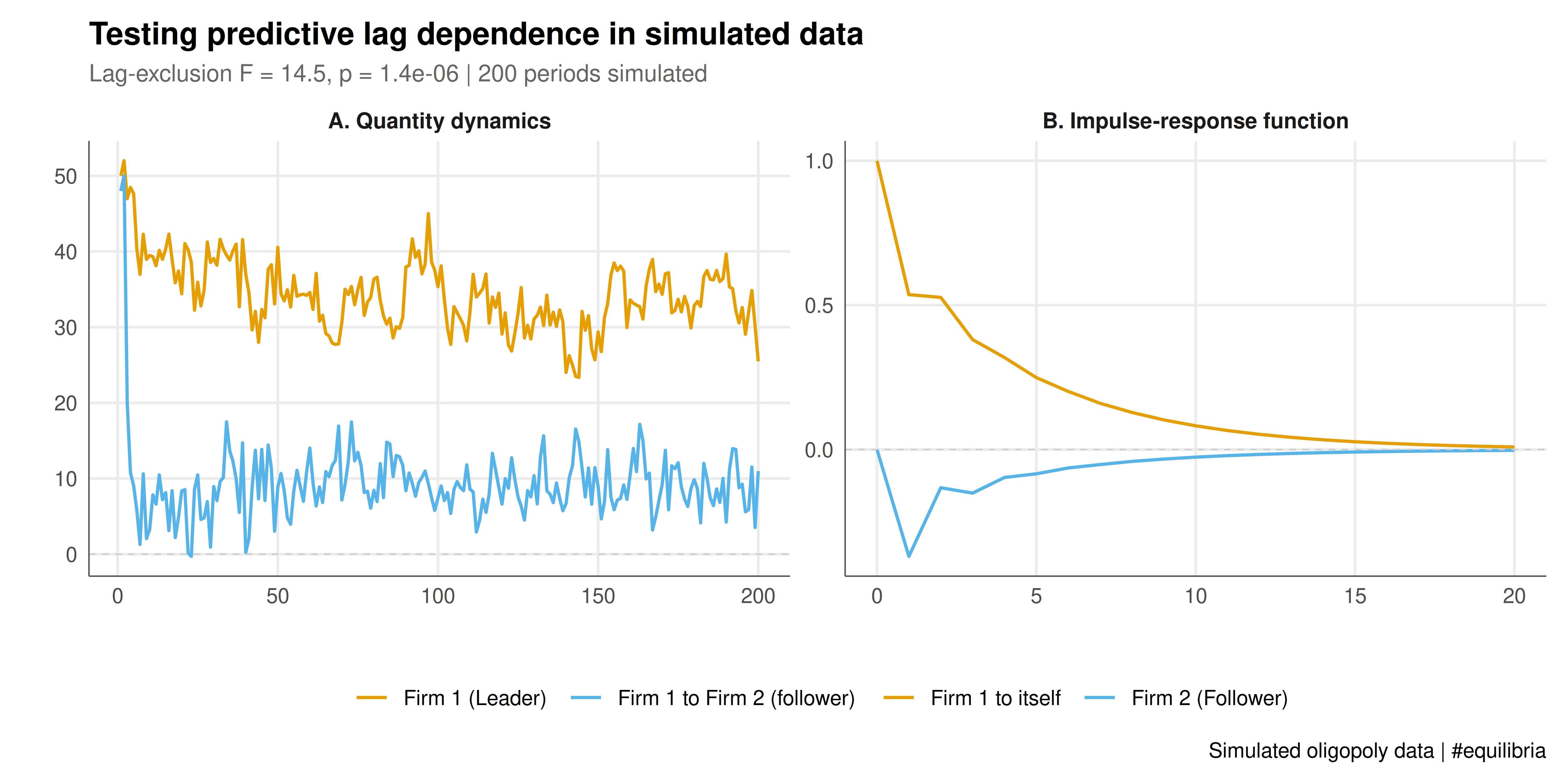
The static figure presents a two-panel comparison: the Stackelberg time series with the Granger causality test results annotated, and the impulse-response functions showing how a shock to the leader propagates to the follower.
```{r}
#| label: fig-granger-causality-static
#| fig-cap: "Figure 1. Granger causality analysis of simulated oligopoly data under Stackelberg competition. Left panel: time series of Firm 1 (leader, orange) and Firm 2 (follower, blue) quantity choices over 200 periods. Right panel: impulse-response functions showing the dynamic effect of a unit shock to Firm 1's output on itself (orange) and on Firm 2 (blue). The cross-response reflects the imposed lag dependence, not identification of Stackelberg competition."
#| dev: [png, pdf]
#| fig-width: 10
#| fig-height: 5
#| dpi: 300
# Panel 1: Time series
ts_data <- data.frame(
  period = rep(1:T_periods, 2),
  quantity = c(q1_stackel, q2_stackel),
  firm = rep(c("Firm 1 (Leader)", "Firm 2 (Follower)"), each = T_periods)
)

p1 <- ggplot(ts_data, aes(x = period, y = quantity, color = firm)) +
  geom_line(alpha = 0.8, linewidth = 0.5) +
  scale_color_manual(values = c(okabe_ito[1], okabe_ito[2]), name = "") +
  annotate("text", x = 100, y = max(ts_data$quantity) * 0.98,
           label = sprintf("Lag exclusion: F1->F2 F=%.1f (p=%.3g)",
                          gc_s_1to2$F_stat, gc_s_1to2$p_value),
           size = 3, color = "grey30") +
  labs(title = "Stackelberg quantity dynamics",
       x = "Period", y = "Quantity") +
  theme_publication() +
  theme(legend.position = "bottom")

# Panel 2: Impulse-response functions
p2 <- ggplot(irf_data, aes(x = horizon, y = response, color = type)) +
  geom_line(linewidth = 1) +
  geom_point(size = 1.5) +
  geom_hline(yintercept = 0, linetype = "dashed", color = "grey50") +
  scale_color_manual(values = c(okabe_ito[1], okabe_ito[2]), name = "") +
  labs(title = "Impulse-response to leader shock",
       x = "Horizon (periods)", y = "Response") +
  theme_publication() +
  theme(legend.position = "bottom")

# Combine panels side by side using a simple approach
# We'll create a combined data plot with faceting
combined_data <- bind_rows(
  ts_data |> transmute(panel = "A. Quantity dynamics",
                     x_val = period, y_val = quantity,
                     group = firm),
  irf_data |> transmute(panel = "B. Impulse-response function",
                      x_val = horizon, y_val = response,
                      group = type)
) |>
  select(x_val, y_val, group, panel)

p_combined <- ggplot(combined_data,
       aes(x = x_val, y = y_val, color = group)) +
  geom_line(linewidth = 0.7) +
  geom_hline(yintercept = 0, linetype = "dashed", color = "grey80",
             linewidth = 0.3) +
  scale_color_manual(
    values = c("Firm 1 (Leader)" = okabe_ito[1],
               "Firm 2 (Follower)" = okabe_ito[2],
               "Firm 1 to itself" = okabe_ito[1],
               "Firm 1 to Firm 2 (follower)" = okabe_ito[2]),
    name = "") +
  facet_wrap(~ panel, scales = "free", nrow = 1) +
  labs(
    title = "Testing predictive lag dependence in simulated data",
    subtitle = sprintf("Lag-exclusion F = %.1f, p = %.3g | 200 periods simulated",
                       gc_s_1to2$F_stat, gc_s_1to2$p_value),
    x = "", y = "",
    caption = "Simulated oligopoly data | #equilibria"
  ) +
  theme_publication() +
  theme(strip.text = element_text(size = 10, face = "bold"))

p_combined
```
## Interactive figure
The interactive version provides hover details for each time point and impulse-response horizon, enabling precise inspection of the dynamic relationship between the two firms.
```{r}
#| label: fig-granger-causality-interactive
# Interactive time series with Granger test annotation
ts_hover <- ts_data |>
  mutate(hover = sprintf("Period: %d\nFirm: %s\nQuantity: %.1f",
                          period,
                          ifelse(firm == "Firm 1 (Leader)", "Firm 1 (Leader)",
                                 "Firm 2 (Follower)"),
                          quantity))

p_ts_int <- ggplot(ts_hover,
       aes(x = period, y = quantity, color = firm, text = hover)) +
  geom_line(alpha = 0.8, linewidth = 0.4) +
  scale_color_manual(values = c(okabe_ito[1], okabe_ito[2]), name = "") +
  labs(title = "Stackelberg dynamics (hover for details)",
       x = "Period", y = "Quantity") +
  theme_publication()

ggplotly(p_ts_int, tooltip = "text") |>
  config(displaylogo = FALSE,
         modeBarButtonsToRemove = c("select2d", "lasso2d", "autoScale2d"))
```
## Interpretation
The printed tests compare prediction with and without cross-series lags in two seeded synthetic examples. Their results depend on the imposed coefficients, sample, lag order and random draws. A non-significant result does not establish the absence of dependence, and a one-directional rejection does not identify economic leadership.
The impulse responses propagate a unit reduced-form innovation through the fitted VAR. Their interpretation as an intervention or structural economic shock requires identification beyond the regressions shown here. The simulation's negative cross-response was built into its coefficient matrix.
For empirical use, check stationarity, lag selection, residual dependence, the conditioning information set and the stability of conclusions across defensible specifications. Short samples and misspecified dynamics can distort inference. This demonstration is not evidence about actual market power, simultaneous play or collusion.
## Extensions & related tutorials
Granger causality is one tool in the broader econometric toolkit for analysing strategic interaction in time-series data. It pairs naturally with VAR estimation, structural break tests, and dynamic game estimation.
- [VAR models for strategic interaction](../../time-series-econometrics/strategic-interaction-var-models/) --- full VAR estimation with model selection, forecasting, and variance decomposition
- [FRED economic data for game-theoretic calibration](../../public-apis-and-datasets/federal-reserve-fred-data/) --- apply Granger tests to real FRED industry data to detect strategic patterns
- [Bootstrap inference for game-theoretic quantities](../../statistical-foundations/bootstrap-game-theory/) --- block bootstrap for Granger test statistics under weak dependence
- [Privacy as a game](../../ethics-applications/privacy-game-theory/) --- time-series analysis of disclosure patterns as strategic sequential moves
## References
::: {#refs}
:::