Interrupted time series for a corpus outcome

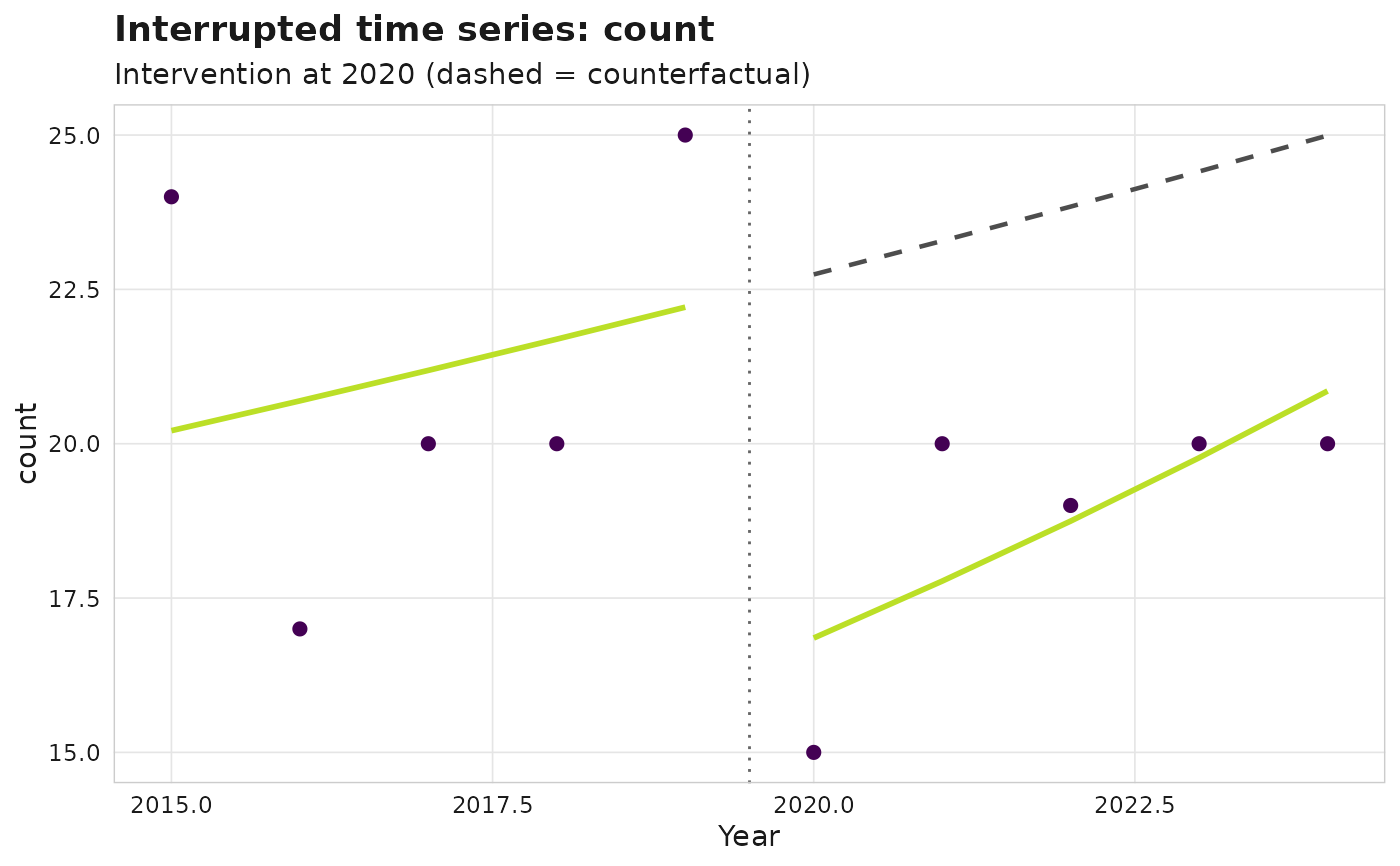
A turnkey interrupted time series (ITS): aggregates the chosen outcome to a yearly series, fits a segmented regression with a level shift and a slope change at intervention_year, and derives the counterfactual (the pre-intervention trend projected forward).

Usage

sm_its(
  corpus,
  intervention_year,
  outcome = c("count", "share_q1", "cnci", "leadership"),
  family = NULL,
  lag = NULL,
  call = rlang::caller_env()
)

# S3 method for class 'sm_its'
print(x, ...)

# S3 method for class 'sm_its'
summary(object, ...)

# S3 method for class 'sm_its'
autoplot(object, ...)

Arguments

corpus

An sm_corpus.

intervention_year

Integer year at which the intervention takes effect.

outcome

One of "count", "share_q1", "cnci", "leadership". The expected source columns are:

"count"

Works per year (uses works$year).

"share_q1"

Share of Q1-journal works; needs a journal-quartile column on works (quartile, jif_quartile, or sjr_quartile).

"cnci"

Mean field-normalised citation impact per year. Impact is resolved from the first populated of works$cnci, a corpus$metrics table (cnci/fnci/value keyed by work_id), or works$cited_by_count (from which FNCI is derived via sm_metric_fnci()). If none is populated, an informative error names the columns inspected.

"leadership"

Share of works with a corresponding/leadership author (uses authorships$is_corresponding).

family

Optional GLM family (a family object, generator function, or name). Defaults to Poisson for "count" and Gaussian otherwise; document your choice when overriding.

lag

Citation-maturity lag in years (default 2). For citation-based outcomes ("cnci"), the most recent lag years are citation-immature and are excluded from the fit; this is reported in the print method.

call

Caller environment for error reporting.

x

An sm_its object.

...

Ignored.

object

An sm_its object.

Value

An sm_its S3 object with components: model (the fitted glm), coefficients (tidy tibble: term, estimate, std.error, conf.low, conf.high, statistic, p.value), series (tibble: year, observed, fitted, counterfactual), and metadata (outcome, intervention_year, family, lag, provisional_years).

print returns x invisibly.

summary returns the tidy coefficient tibble.

autoplot returns a ggplot.

See also

sm_did(), sm_citation_maturity()

Other causal: sm_did(), sm_synth()

Examples

corpus <- sm_example_corpus(n_works = 200, seed = 1)
its <- sm_its(corpus, intervention_year = 2020, outcome = "count")
its
#> 
#> ── <sm_its> ────────────────────────────────────────────────────────────────────
#> Outcome: count Family: poisson
#> Intervention year: 2020
#> 
#> 
#> ── Segmented regression coefficients 
#> Baseline level: 3.0063 [2.6712, 3.3413] (p = <2e-16)
#> Pre-trend (slope): 0.0236 [-0.1111, 0.1583] (p = 0.73)
#> Level change: -0.2997 [-0.8709, 0.2714] (p = 0.3)
#> Slope change: 0.0297 [-0.1669, 0.2262] (p = 0.77)
# \donttest{
ggplot2::autoplot(its)

# }