Hyperspectral Tissue Characterization
Can tissue regions be told apart by their reflectance spectra alone, and which spectral features separate them?
Data: Two sources, both synthetic. The example recording bundled with tivis.r (12 × 16 pixels, 8 bands at 500–535 nm), a generated cube written in the real TIVITA SpecCube.dat layout; and six 60 × 80-pixel tissue scenes simulated in this walkthrough (seeded) on the TIVITA wavelength grid (500–995 nm in 5 nm steps) from the Prahl hemoglobin extinction table that ships with hyperspectR. No patient, cohort or project data.


hyperloomInstall the suite
tivis.rRead a TIVITA recording

cuvis.rCheck the Cubert SDK- Simulate tissue scenes

hyperspectRSmooth and normalise-
hyperspectRHemoglobin fit and band ratios -
hyperspectREmbedding and classification 

hyperspectaculRSpectral summaries
A hyperspectral camera records a reflectance spectrum at every pixel. This walkthrough follows one path through the CTTIR hyperspectral suite: read a recording, preprocess the cube, fit hemoglobin, reduce and classify the spectra, and summarise them visually. The tissue scenes are simulated, so the right answer is known in advance. That is deliberate: it lets us check what each step recovers and where it goes wrong.
Install the suite Link to heading
hyperloom installs the four member packages and their dependencies. It has
no functions of its own and attaches nothing, so the members are loaded
directly.
# remotes::install_github("CTTIR/hyperloom")
trimws(strsplit(packageDescription("hyperloom")$Imports, ",")[[1]])
#> [1] "hyperspectR" "hyperspectaculR" "cuvis.r" "tivis.r"
library(tivis.r)
library(cuvis.r)
library(hyperspectR)
library(hyperspectaculR)
library(ggplot2)
library(patchwork)
Read a TIVITA recording Link to heading
The Diaspective TIVITA Suite stores each capture as a binary
*_SpecCube.dat file next to a *_meta.log. tivis.r reads both in pure R.
The header is read first, without touching the samples:
f <- tivis_example_file()
basename(f)
#> [1] "example_SpecCube.dat"
str(tivis_read_header(f))
#> List of 5
#>  $ width    : int 16
#>  $ height   : int 12
#>  $ bands    : int 8
#>  $ n_values : num 1536
#>  $ file_size: num 6156
meta <- tivis_get_metadata(sub("_SpecCube[.]dat$", "_meta.log", f))
meta$Aufnahme$Aufnahmemodus
#> [1] "Reflektanz"
hs_read_tivita() calls the same reader and returns an hsi_cube, the class
that the rest of the suite works on. It carries the wavelengths, a pixel mask
and the acquisition metadata.
rec <- hs_read_tivita(f, verbose = FALSE)
rec
hs_plot_image(rec, wavelength = 515) + hs_plot_spectra(rec)
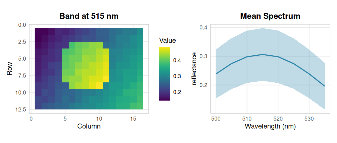
The bundled recording at 515 nm and its mean spectrum (± 1 SD): a smooth gradient with a bright disc, read through the real TIVITA parser.
A full TIVITA cube has 100 bands and is roughly 123 MB. The bundled file is a small fixture with only the first eight bands: enough to exercise the parser, too narrow for tissue indices. The rest of the walkthrough therefore uses simulated scenes on the full TIVITA wavelength grid.
Check the Cubert SDK Link to heading
Cubert snapshot cameras write .cu3s session files that only the vendor’s
CUVIS SDK can decode. cuvis.r binds that SDK, and hs_read_cubert() uses it
to return the same hsi_cube class as the TIVITA reader. No session file ships
with the packages, so here we only confirm that the SDK is linked and list the
processing modes a recording can be reprocessed into.
cuvis_available()
#> [1] TRUE
if (cuvis_available()) cuvis_version()
#> [1] "CUBERT SDK v. 3.5.3 build: 0f416fb6327f26644290b554c9b16050a515b89d"
cuvis_processing_modes
#>              Raw     DarkSubtract      Reflectance SpectralRadiance
#>                0                1                2                3
#>          Preview
#>                5
Simulate tissue scenes Link to heading
Each scene is an elliptical field of tissue on a dark drape. Four tissue types differ only in three parameters: the oxygenated fraction of hemoglobin, total hemoglobin and a scattering factor.
tissue <- data.frame(
  class   = c("perfused", "hypoxic", "congested", "pale"),
  sto2    = c(0.80, 0.35, 0.60, 0.75),   # HbO2 / (HbO2 + Hb)
  thb_uM  = c(60, 60, 160, 15),          # total hemoglobin, µmol/L
  scatter = c(1.00, 1.00, 0.90, 1.35)
)
tissue
#>       class sto2 thb_uM scatter
#> 1  perfused 0.80     60    1.00
#> 2   hypoxic 0.35     60    1.00
#> 3 congested 0.60    160    0.90
#> 4      pale 0.75     15    1.35
Reflectance follows a simple Beer–Lambert model on a sloping scattering
baseline, with an optical path that lengthens into the near infrared. The
extinction coefficients are the tabulated values from hs_chromophore_data()
and the wavelength grid comes from tivis_get_wavelengths(). Region borders
are blurred, every pixel gets its own jitter, and illumination falls off from a
random hot spot. Scenes differ in layout, illumination and a scene-wide shift
in oxygenation.
wl  <- tivis_get_wavelengths(100L)                      # 500-995 nm
ext <- hs_chromophore_data(c("HbO2", "Hb"), wavelength_range = c(500, 996))
eps_o <- approx(ext$wavelength, ext$HbO2, wl)$y         # cm^-1 / (mol/L)
eps_d <- approx(ext$wavelength, ext$Hb, wl)$y

blur <- function(m, k = 5) {
  sm <- function(v) { s <- stats::filter(v, rep(1 / k, k)); ifelse(is.na(s), v, s) }
  apply(t(apply(m, 1, sm)), 2, sm)
}

simulate_scene <- function(seed, rows = 60, cols = 80) {
  set.seed(seed)
  y <- row(matrix(0, rows, cols)); x <- col(matrix(0, rows, cols))
  blob <- function(cx, cy, rx, ry) ((x - cx) / rx)^2 + ((y - cy) / ry)^2 < 1
  field <- blob(cols / 2, rows / 2, 0.47 * cols, 0.46 * rows)
  truth <- matrix("perfused", rows, cols)
  truth[blob(runif(1, 20, 60), runif(1, 15, 45), runif(1, 10, 16), runif(1, 8, 13))] <- "hypoxic"
  truth[blob(runif(1, 20, 60), runif(1, 15, 45), runif(1, 6, 10), runif(1, 6, 10))] <- "congested"
  truth[blob(runif(1, 15, 65), runif(1, 15, 45), runif(1, 4, 7), runif(1, 10, 18))] <- "pale"
  truth[!field] <- NA

  p <- tissue[match(truth, tissue$class), ]
  sto2 <- blur(matrix(p$sto2, rows)) + rnorm(1, 0, 0.04) + rnorm(rows * cols, 0, 0.03)
  sto2 <- pmin(pmax(sto2, 0), 1)
  thb  <- blur(matrix(p$thb_uM, rows)) * exp(rnorm(rows * cols, 0, 0.10))
  sca  <- blur(matrix(p$scatter, rows))
  light <- 1 - 1.4 * ((x - runif(1, 25, 55))^2 + (y - runif(1, 20, 40))^2) / (rows^2 + cols^2)

  path_cm  <- 0.06 * (wl / 500)^3              # longer light paths in the NIR
  baseline <- 0.40 + 0.15 * (wl - 500) / 495   # scattering background
  data <- array(0.03, c(rows, cols, length(wl)))
  for (i in which(field)) {
    mua <- 1e-6 * thb[i] * (sto2[i] * eps_o + (1 - sto2[i]) * eps_d)
    data[row(field)[i], col(field)[i], ] <- light[i] * sca[i] * baseline * 10^(-mua * path_cm)
  }
  data <- data + rnorm(length(data), 0, 0.004)
  sto2[!field] <- NA
  list(cube  = hsi_cube(data, wl, mask = field,
                        metadata = list(processing_mode = "reflectance")),
       truth = truth, sto2 = sto2)
}

scenes <- lapply(1:6, simulate_scene)
scene  <- scenes[[1]]
scene$cube
table(scene$truth)
#>
#> congested   hypoxic      pale  perfused
#>       262       356       150      2485
class_colours <- c(perfused = "#CC3311", hypoxic = "#0077BB",
                   congested = "#882255", pale = "#DDCC77")
show_map <- function(m, title) {
  df <- data.frame(row = as.vector(row(m)), col = as.vector(col(m)),
                   class = factor(as.vector(m), levels = names(class_colours)))
  ggplot(df, aes(col, row, fill = class)) + geom_raster() +
    scale_fill_manual(values = class_colours, breaks = names(class_colours),
                      na.value = "grey85", drop = FALSE) +
    scale_y_reverse() + coord_equal() + labs(title = title, x = NULL, y = NULL) +
    theme_hsi()
}
hs_plot_rgb(scene$cube, r = 640, g = 550, b = 500) + show_map(scene$truth, "Simulated classes")
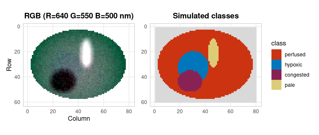
Scene 1 as a pseudo-colour image (left) and the classes it was simulated from (right, grey = drape). The pale stripe is bright and the congested patch dark; the hypoxic region is hard to see by eye.
Smooth and normalise Link to heading
Preprocessing is written as a recipe, so exactly the same steps can be re-applied to held-out data later: a Savitzky–Golay filter (7 bands, quadratic) followed by standard normal variate (SNV) scaling, which removes the brightness differences caused by uneven illumination. The filter only returns bands with a full window, so three bands are lost at each end.
recipe <- hs_recipe(list(
  list(method = "smooth", args = list(window = 7L, poly = 2L)),
  list(method = "snv")
))
snv <- hs_process(scene$cube, recipe)$cube
range(snv$wavelengths)
#> [1] 515 980
snv$metadata$processing_mode
#> [1] "snv"
class_spectra <- function(cube, truth, step) {
  do.call(rbind, lapply(tissue$class, function(k) {
    s <- hs_roi_stats(cube, !is.na(truth) & truth == k)
    data.frame(step = step, class = k, wavelength = s$wavelength, mean = s$mean, sd = s$sd)
  }))
}
spec <- rbind(class_spectra(scene$cube, scene$truth, "Reflectance"),
              class_spectra(snv, scene$truth, "Smoothed + SNV"))
ggplot(spec, aes(wavelength, mean, colour = class, fill = class)) +
  geom_ribbon(aes(ymin = mean - sd, ymax = mean + sd), alpha = 0.15, colour = NA) +
  geom_line(linewidth = 0.7) +
  facet_wrap(~step, scales = "free_y") +
  scale_colour_manual(values = class_colours, aesthetics = c("colour", "fill")) +
  labs(x = "Wavelength (nm)", y = NULL) + theme_hsi()
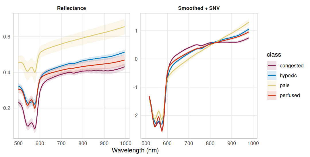
Class mean spectra ± 1 SD before and after preprocessing. Raw reflectance mixes tissue type with illumination; after SNV the classes differ in shape, around the 540/575 nm hemoglobin bands, between 600 and 800 nm and in the slope into the near infrared.
Hemoglobin fit and band ratios Link to heading
hs_beer_lambert() converts reflectance to absorbance and fits the HbO2 and
Hb extinction spectra between 500 and 600 nm by non-negative least squares;
hs_sto2() returns the fitted HbO2 fraction. hs_npi() and hs_thi() are
dimensionless band ratios. hs_plot_clinical() puts them next to an RGB view
and masks the drape by its low reflectance.
hs_plot_clinical(scene$cube, indices = c("sto2", "npi", "thi"), ncol = 2)
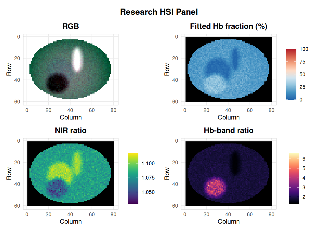
Fitted HbO2 fraction and two band ratios for scene 1. The congested patch stands out in every panel; the hypoxic and pale regions both read as a low fitted fraction.
Because the scene is simulated, the fitted fraction can be checked against the value that generated each pixel:
fit <- hs_beer_lambert(scene$cube)
cmp <- data.frame(class     = as.vector(scene$truth),
                  simulated = 100 * as.vector(scene$sto2),
                  fitted    = as.vector(fit$sto2))
cmp <- cmp[!is.na(cmp$class), ]
aggregate(cbind(simulated, fitted) ~ class, data = cmp,
          FUN = function(v) round(median(v), 1))
#>       class simulated fitted
#> 1 congested      62.6   26.6
#> 2   hypoxic      40.0    3.8
#> 3      pale      77.8    4.8
#> 4  perfused      81.5   16.5
ggplot(cmp, aes(simulated, fitted, colour = class)) +
  geom_abline(linetype = 2, colour = "grey50") +
  geom_point(size = 0.6, alpha = 0.4) +
  scale_colour_manual(values = class_colours) +
  guides(colour = guide_legend(override.aes = list(size = 2, alpha = 1))) +
  coord_equal(xlim = c(0, 100), ylim = c(0, 100)) +
  labs(x = "Simulated HbO2 fraction (%)", y = "Fitted HbO2 fraction (%)") + theme_hsi()
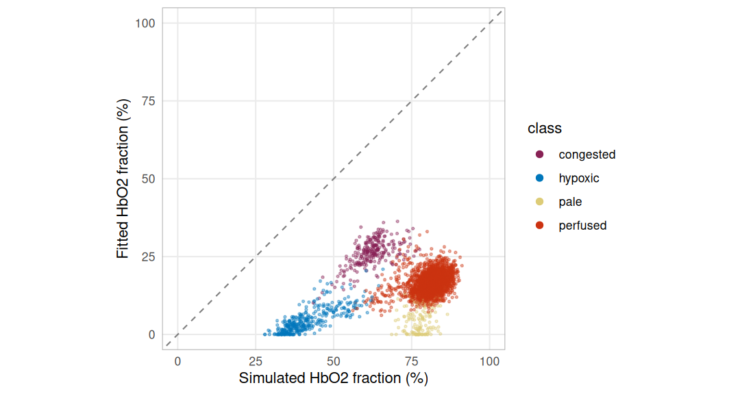
Fitted against simulated HbO2 fraction per pixel; the dashed line is perfect agreement. The fit sits far below it, and lowest where there is least hemoglobin.
The fit has no term for the scattering background, so the flat part of the absorbance is taken up by the hemoglobin spectra, mostly by deoxyhemoglobin. The less hemoglobin a pixel holds, the larger that bias: the pale class, simulated at 75 %, comes out near the hypoxic one. The package documentation describes the output as a research model estimate for this reason. Read it as a relative, model-bound number, not as tissue oxygen saturation.
Embedding and classification Link to heading
Unsupervised: PCA and k-means Link to heading
PCA on the preprocessed cube gives a low-dimensional embedding whose loadings are spectra and can be read directly. Clustering the first three scores asks whether the classes emerge without labels.
pca <- hs_pca(snv, n_components = 3)
round(100 * pca$variance_explained, 1)
#> [1] 74.6 10.9 1.6
scores <- matrix(pca$scores, ncol = 3, dimnames = list(NULL, paste0("PC", 1:3)))
ok <- complete.cases(scores)
aggregate(round(scores[ok, ], 2), by = list(class = scene$truth[ok]), FUN = median)
#>       class   PC1   PC2   PC3
#> 1 congested -1.20  0.49  0.15
#> 2   hypoxic  0.57  0.52 -0.13
#> 3      pale  2.07  0.05  0.18
#> 4  perfused -0.08 -0.13 -0.01
round(cor(scores[ok, ], scene$sto2[ok])[, 1], 2) # with the simulated HbO2 fraction
#>   PC1   PC2   PC3
#> -0.13 -0.92  0.28
PC1 orders the classes from pale to congested, so it mainly follows how much hemoglobin absorbs; its loading sets the 540–575 nm bands and the near infrared against the 600–800 nm range. PC2 correlates strongly with the simulated oxygenation. Its loading has peaks at 540 and 575 nm, the two oxyhemoglobin bands, and a trough at 555–560 nm, where deoxyhemoglobin has its single band. The embedding is readable because its axes are spectra.
set.seed(1)
km <- kmeans(scores[ok, ], centers = 4, nstart = 20)
table(simulated = scene$truth[ok], cluster = km$cluster)
#>            cluster
#> simulated      1    2    3    4
#>   congested    4    0    0  258
#>   hypoxic     22    0  327    7
#>   pale         1  105   44    0
#>   perfused  2320    0  132   33
loadings <- data.frame(wavelength = rep(snv$wavelengths, 3),
                       loading = as.vector(pca$loadings),
                       component = rep(paste0("PC", 1:3), each = length(snv$wavelengths)))
cluster_map <- matrix(NA_integer_, nrow(scene$truth), ncol(scene$truth))
cluster_map[ok] <- km$cluster
p_load <- ggplot(loadings, aes(wavelength, loading, colour = component)) +
  geom_hline(yintercept = 0, colour = "grey70") + geom_line(linewidth = 0.7) +
  scale_colour_manual(values = c(PC1 = "#222222", PC2 = "#EE7733", PC3 = "#009988")) +
  labs(x = "Wavelength (nm)", y = "Loading", colour = NULL) + theme_hsi()
p_clus <- ggplot(data.frame(row = as.vector(row(cluster_map)), col = as.vector(col(cluster_map)),
                            cluster = factor(as.vector(cluster_map))),
                 aes(col, row, fill = cluster)) + geom_raster() +
  scale_fill_brewer(palette = "Set2", breaks = as.character(1:4), na.value = "grey85") +
  scale_y_reverse() + coord_equal() + labs(title = "k-means on PC1-3", x = NULL, y = NULL) +
  theme_hsi()
p_load + p_clus + plot_layout(widths = c(1.2, 1))
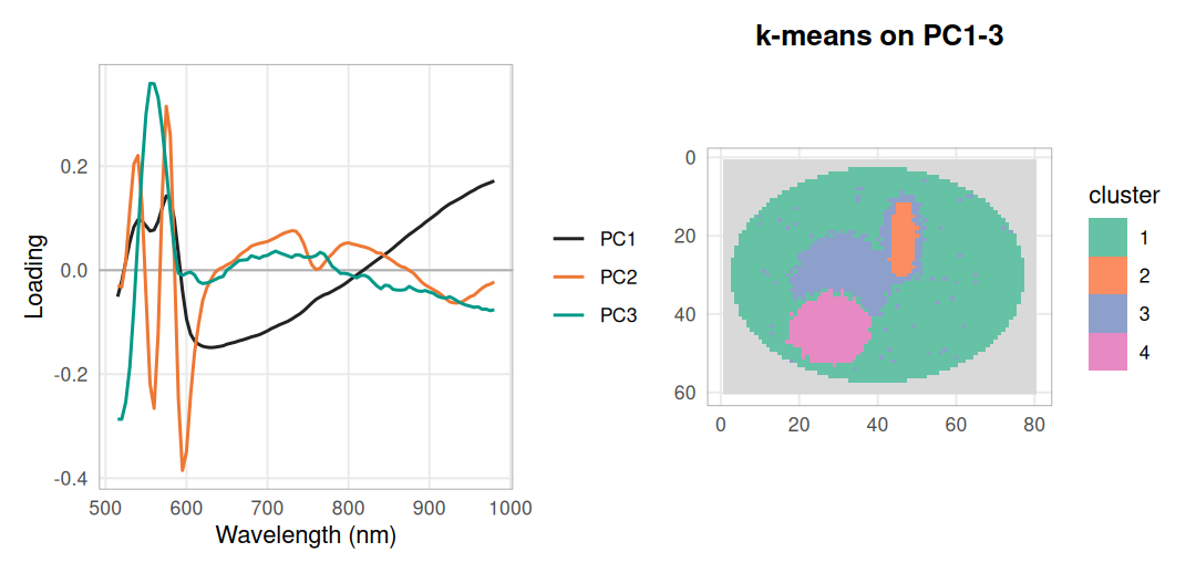
PCA loadings (left) and four k-means clusters on the first three scores (right). The clusters follow the simulated regions, with mixed pixels along the blurred borders and part of the pale stripe joining the hypoxic cluster.
Supervised, with whole scenes held out Link to heading
Pixels from one image are not independent, so a classifier must be tested on
scenes it has never seen. hs_grouped_evaluate() does this: it fits the recipe
and the classifier on five scenes and predicts the sixth, in turn for each
scene. Sixty pixels per class are sampled from every scene.
set.seed(3)
px <- lapply(seq_along(scenes), function(s) {
  lab <- as.vector(scenes[[s]]$truth)
  idx <- unlist(lapply(split(which(!is.na(lab)), lab[!is.na(lab)]),
                       function(v) v[sample.int(length(v), 60)]))
  list(x = matrix(scenes[[s]]$cube$data, ncol = length(wl))[idx, ],
       label = lab[idx], scene = rep(paste("scene", s), length(idx)))
})
spectra <- do.call(rbind, lapply(px, `[[`, "x"))
labels  <- unlist(lapply(px, `[[`, "label"))
groups  <- unlist(lapply(px, `[[`, "scene"))

ev <- hs_grouped_evaluate(spectra, wl, labels, groups, n_folds = 6,
                          method = "svm", recipe = recipe, bootstrap = 500)
round(c(accuracy = ev$accuracy, lower = ev$accuracy_interval[1],
        upper = ev$accuracy_interval[2], balanced = ev$balanced_accuracy), 3)
#> accuracy    lower    upper balanced
#>    0.958    0.945    0.971    0.958
ev$confusion
#>            predicted
#> observed    congested hypoxic pale perfused
#>   congested       354       2    0        4
#>   hypoxic           5     349    2        4
#>   pale              2       5  336       17
#>   perfused          7       8    4      341
The interval resamples whole scenes, not pixels. With six scenes it is narrow only because the simulated scenes are alike.
To see where the errors fall, the same recipe and an SVM are fitted on the
sampled pixels of scenes 1–5 and applied to every pixel of scene 6.
hs_predict() checks that the new cube went through the same preprocessing.
train <- groups != "scene 6"
train_cube <- hsi_cube(array(spectra[train, ], c(sum(train), 1, length(wl))), wl,
                       metadata = list(processing_mode = "reflectance"))
fitted <- hs_process(train_cube, recipe)
model  <- hs_classify_svm(fitted$cube, matrix(labels[train], ncol = 1))
test   <- hs_process(scenes[[6]]$cube, fitted$recipe, learn = FALSE)$cube
pred   <- hs_predict(model, test)
round(mean(pred == scenes[[6]]$truth, na.rm = TRUE), 3)
#> [1] 0.945
wrong <- pred
wrong[!is.na(pred) & pred == scenes[[6]]$truth] <- NA
show_map(scenes[[6]]$truth, "Scene 6: simulated") +
  show_map(pred, "Predicted") +
  show_map(wrong, "Misclassified") +
  plot_layout(guides = "collect")
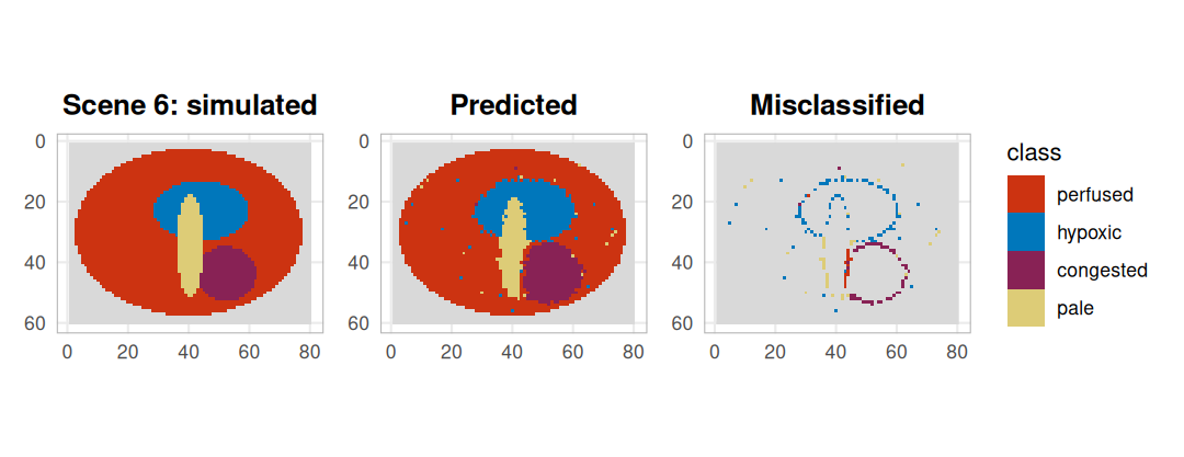
The held-out scene: simulated classes, SVM prediction, and the misclassified pixels coloured by their wrong prediction. Errors sit along region borders, where blurred parameters give spectra between two classes.
Spectral summaries Link to heading
hyperspectaculR renders a cube as images that describe its values, and
records what it selected and how it stretched them. A three-channel fusion
maps near-infrared, red and green bands to R, G and B; the spectral density
shows how reflectance is distributed in every band across the tissue pixels.
Both plots carry a long caption with these details; it is dropped here for
space, and the full record stays available through hsa_provenance(). The
masked drape is left transparent.
fusion <- hsa_fusion(scene$cube, red = c(800, 850, 900), green = c(620, 660, 700),
                     blue = c(540, 560, 580), by = "wavelength")
density <- hsa_spectral_density(scene$cube, nbins = 64, normalise = "band",
                                value_label = "reflectance")
fusion + labs(caption = NULL) + density + labs(caption = NULL) +
  plot_layout(widths = c(1, 1.3))
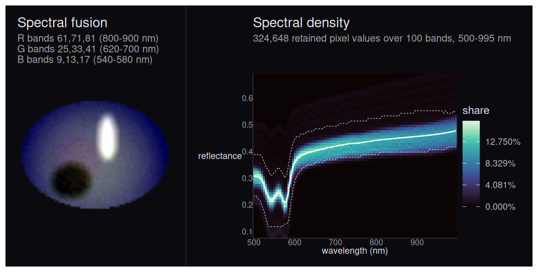
False-colour fusion of scene 1 (left) and the per-band distribution of tissue reflectance (right, white line = binned mean, dashed = 5-95 % envelope). The pale stripe and the congested patch form faint ridges above and below the main band.
sapply(hsa_provenance(fusion)$selection[c("red", "green", "blue")], `[[`, "coordinates")
#>      red green blue
#> [1,] 800   620  540
#> [2,] 850   660  560
#> [3,] 900   700  580
What this shows, and its limits Link to heading
The suite carries one object, hsi_cube, from file readers through a
recorded preprocessing recipe to embeddings, classifiers and figures. On the
simulated scenes, four tissue types were separable from their spectra alone.
K-means on three principal components recovered the regions without labels.
An SVM on smoothed, SNV-scaled spectra reached
95.8 % accuracy with whole scenes held out, and
94.5 % on every
tissue pixel of scene 6; the errors sit on region borders. Two spectral
features carry the separation: overall hemoglobin absorption (PC1, pale
against congested) and the shape of the 540–575 nm hemoglobin bands (PC2,
oxygenation).
The limits are as important. The data are simulated from a simple forward
model, and the same extinction table drives simulation and fitting, so
these numbers say the pipeline works, not that tissue can be classified.
Real recordings add specular highlights, motion, camera noise and tissue
types that do not follow four parameter sets. The fitted HbO2 fraction is
strongly biased by scattering and should not be read as oxygen saturation.
Neither the TIVITA fixture nor the Cubert check involved a real capture. A
real study would label regions on recordings from independent patients and
pass the patient as the group to hs_grouped_evaluate().
Package versions Link to heading
pkgs <- c("hyperloom", "tivis.r", "cuvis.r", "hyperspectR", "hyperspectaculR")
knitr::kable(data.frame(
  package = pkgs,
  version = vapply(pkgs, function(p) as.character(packageVersion(p)), ""),
  commit  = vapply(pkgs, function(p) packageDescription(p)$RemoteSha %||% NA_character_, "")
), row.names = FALSE)
| package | version | commit |
|---|---|---|
| hyperloom | 0.1.1 | bfd38304aa1e89e783a904172070511d2485868f |
| tivis.r | 0.1.0 | 1a28d08f8a24fbeaed0e353ba81aa20f5f36831a |
| cuvis.r | 0.1.0 | 89bb9c2a0b7480414e375db4a89097143e32c846 |
| hyperspectR | 0.2.0.9000 | 09170d23b7c4191e550e2f8eb78868e8d2c3a087 |
| hyperspectaculR | 0.2.0 | eb3067ad4e2101db0b1f2d820cf4d9d1715d9f5f |