
cr_dose_response() fits three standard models to
unit-level summaries of one channel across exposure levels:
-
4PL — four-parameter logistic in
log10(dose), with a free lower asymptote; - 3PL — the same shape with the lower asymptote fixed at zero;
-
linear —
y ~ x, for a readout that has no plateau in the range measured.
Setting up an exposure axis
Any cr_experiment whose design carries a
numeric dose column is eligible. The demonstration
experiment has one already, but its levels are tied to treatment names
rather than spread along an axis, so we widen it into six exposure
levels.
exp <- cr_example_experiment(seed = 3, n_cells_per_well = 60)

exp$design$dose <- c(Untreated      = 1,
                     CompoundB      = 10,
                     CompoundC      = 30,
                     CompoundA_low  = 100,
                     CompoundA_high = 300,
                     PosControl     = 1000)[exp$design$treatment]

table(exp$design$dose)
#>
#>    1   10   30  100  300 1000
#>   16   16   16   16   16   16
Doses must be strictly positive when log_dose = TRUE; a
zero-dose vehicle level has no place on a log axis, and the function
drops such units rather than taking log10(0).
Fitting
marker_2 is the readout that falls as exposure rises,
which is the shape a half-maximal inhibitory concentration
describes.
fit <- cr_dose_response(exp,
                        channel  = "marker_2",
                        model    = "4pl",
                        log_dose = TRUE)
fit$model
#> [1] "4pl"
fit$params
#> # A tibble: 4 × 3
#>   parameter estimate std_error
#>   <chr>        <dbl>     <dbl>
#> 1 a           767.     14.0
#> 2 d           326.     24.3
#> 3 e             2.10    0.0566
#> 4 b             8.11    3.74
a is the upper asymptote, d the lower,
e the inflection point on the log10(dose)
scale and b the slope there.
IC50 / EC50
cr_ic50(fit)
#> # A tibble: 1 × 5
#>   parameter estimate ci_low ci_high units
#>   <chr>        <dbl>  <dbl>   <dbl> <chr>
#> 1 IC50          125.   96.6    161. uM
The estimate is back-transformed to the dose scale, with the interval
carried through from the standard error of e.
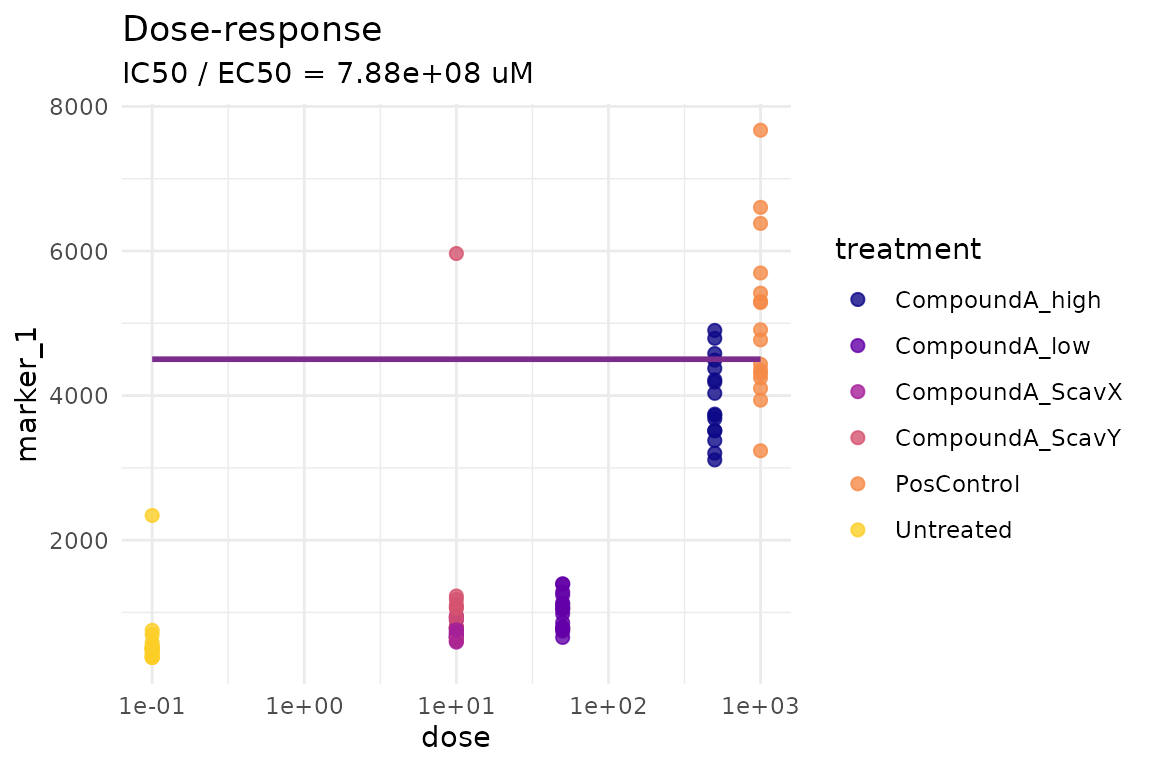
Comparing models
Fixing the lower asymptote at zero moves the inflection point, and with it the IC50 — a reminder that the number is a property of the model as much as of the data:
Checking that the fit converged
cr_dose_response() calls stats::nls() with
warnOnly = TRUE, so a fit that runs out of iterations is
returned rather than raised. Two checks catch it:
-
fit$modelis"linear"instead of the model you asked for whennls()failed outright and the linear fallback took over. -
std_errorisNAfor every parameter whennls()returned without converging. The point estimates from such a fit should not be quoted, and neither should the IC50 derived from them.
A readout that rises with exposure is the usual cause. The logistic is fitted from starting values that describe a falling curve, so an increasing response often does not converge. Fit the channel that falls, or use the linear model:
lin <- cr_dose_response(exp, channel = "marker_1", model = "linear")
lin$params
#> # A tibble: 2 × 2
#>   parameter estimate
#>   <chr>        <dbl>
#> 1 intercept    -370.
#> 2 slope        1488.
Here the slope is the change in the unit-level median of
marker_1 per tenfold increase in exposure.
Where this fits
vignette("end-to-end") runs the full screening pipeline,
in which the exposure axis is handled as a set of contrasts against the
vehicle of each unit’s own batch rather than as a fitted curve. Curve
fitting is the right tool when the exposure levels are dense enough to
define a shape; contrasts are the right tool when they are not.