library(tidyverse)
library(palmerpenguins)
library(patchwork)
set.seed(42)
theme_set(theme_minimal(base_size = 12))Week 1, Session 5 — ggplot2 grammar and multi-panel layouts
Course 1 — #courses
Note
Workflow labs use the variant template: Goal → Approach → Execution → Check → Report.
Learning objectives
- Build a ggplot by naming data, aesthetics, geoms, and scales rather than by calling a plot type.
- Use faceting to display the same relationship across subgroups.
- Combine several plots into a single figure with patchwork.
Prerequisites
Labs 1.2 through 1.4.
Background
ggplot2 is built on a grammar of graphics. Rather than call a function named “scatterplot” or “boxplot”, you declare what the plot contains: a dataset, mappings from variables to aesthetics (x, y, colour, size, shape), and one or more geoms that render those mappings. The result is that any plot you can picture can be built by the same small vocabulary. Once the vocabulary is second nature, you will spend less time searching for a plotting function and more time thinking about what the graph should show.
Multi-panel figures are the standard unit of publication. Faceting breaks one plot into small multiples — the same relationship repeated across a grouping variable — which is almost always a better answer than crowding more colours onto a single panel. The patchwork package takes independent ggplots and assembles them into a single figure using +, |, and / operators, so you can build a three-panel manuscript figure without leaving R.
A common beginner mistake is to treat ggplot as a collection of geom_* functions. It is cleaner to think of a plot as a data-plus- aesthetics object to which geoms are added. Changing the underlying data is then a substitution, not a rewrite.
Setup
1. Goal
Build a three-panel figure that describes bill morphology and body mass in the penguins dataset, using a scatter plot, a boxplot, and a faceted scatter plot, assembled with patchwork.
2. Approach
p <- penguins |>
  drop_na(bill_length_mm, bill_depth_mm, body_mass_g, species, sex)
The plot object is built in three lines: data, aesthetics, geom.
p1 <- p |>
  ggplot(aes(bill_length_mm, bill_depth_mm, colour = species)) +
  geom_point(alpha = 0.7) +
  labs(x = "Bill length (mm)",
       y = "Bill depth (mm)",
       colour = NULL)
p1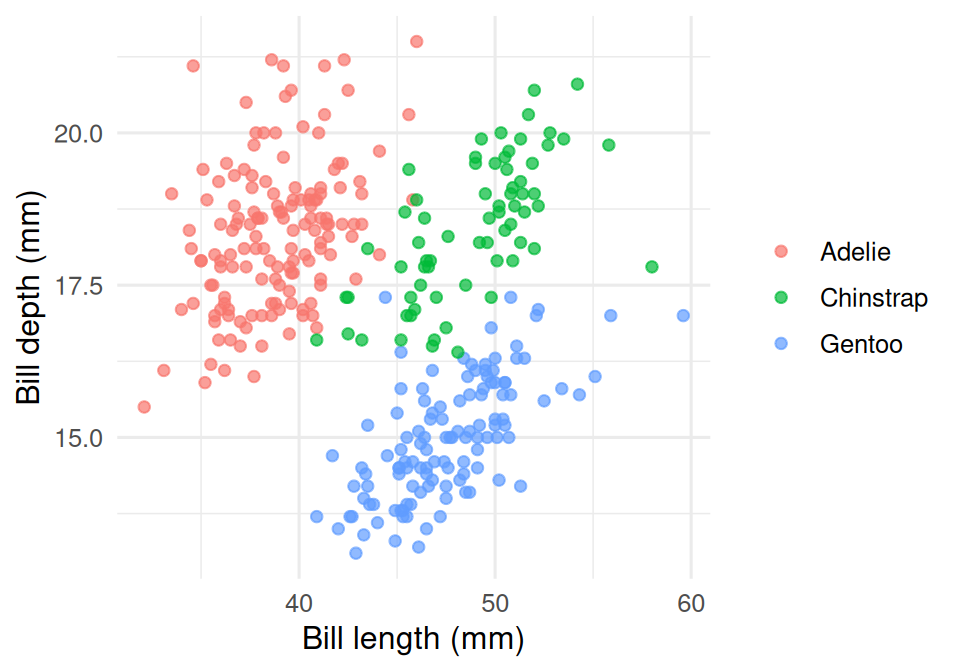
3. Execution
p2 <- p |>
  ggplot(aes(species, body_mass_g, fill = species)) +
  geom_boxplot(alpha = 0.6, colour = "grey30") +
  labs(x = NULL, y = "Body mass (g)") +
  theme(legend.position = "none")
p2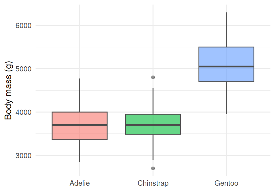
p3 <- p |>
  ggplot(aes(bill_length_mm, body_mass_g, colour = sex)) +
  geom_point(alpha = 0.6) +
  facet_wrap(~ species) +
  labs(x = "Bill length (mm)",
       y = "Body mass (g)",
       colour = NULL)
p3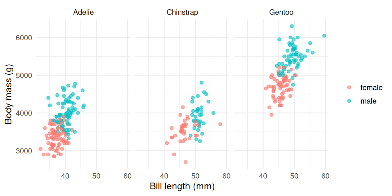
Faceting shows the same relationship in three panels, one per species. The within-species slopes are visually separable from the between-species differences.
4. Check
Assemble the three panels with patchwork.
(p1 | p2) / p3 +
  plot_annotation(
    title = "Palmer penguins: bill morphology and body mass",
    tag_levels = "A"
  )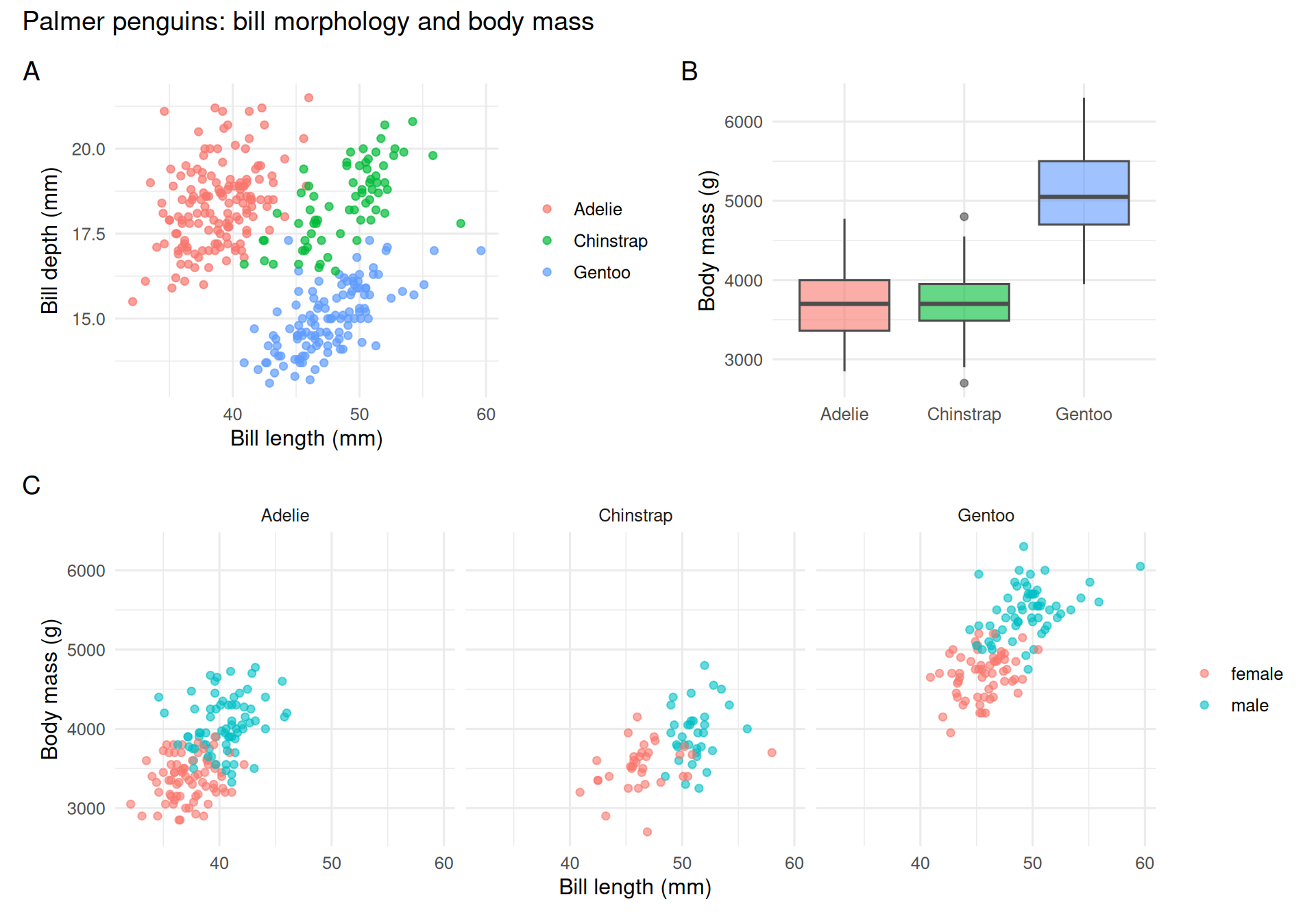
The layout operators: | places side-by-side, / stacks, + groups. plot_annotation() adds title and the familiar A/B/C labels used in manuscripts.
5. Report
A three-panel figure was assembled from the
palmerpenguinsdata (n = 333 complete cases) using ggplot2 and patchwork. Panel A shows a clear separation of bill morphology among the three species. Panel B shows Gentoo as markedly heavier than the other two. Panel C, faceted by species, reveals a within-species positive association between bill length and body mass, with a sex offset visible in each panel.
Within-group and between-group variation are separate features of the data. Faceting is the simplest way to let a reader see both at once.
Live-build the figure one geom at a time, adding the facet at the end. Resist the temptation to show a finished plot straight away; the pedagogy is in watching a plot grow.
Common pitfalls
- Using colour to encode more than one thing at a time (group and magnitude — pick one).
- Mapping a continuous variable to shape.
- Overlaying more than four or five categories on a single scatter plot; use faceting instead.
- Defaulting to
theme_grey(); the in-house convention istheme_minimal(base_size = 12).
Further reading
- Wickham H. ggplot2: Elegant Graphics for Data Analysis, chapters on the grammar and on faceting.
- Pedersen T. patchwork package documentation.
Session info
sessionInfo()R version 4.5.2 (2025-10-31 ucrt)
Platform: x86_64-w64-mingw32/x64
Running under: Windows 11 x64 (build 26200)
Matrix products: default
LAPACK version 3.12.1
locale:
[1] LC_COLLATE=English_Germany.utf8 LC_CTYPE=English_Germany.utf8
[3] LC_MONETARY=English_Germany.utf8 LC_NUMERIC=C
[5] LC_TIME=English_Germany.utf8
time zone: Europe/Berlin
tzcode source: internal
attached base packages:
[1] stats graphics grDevices utils datasets methods base
other attached packages:
[1] patchwork_1.3.2 palmerpenguins_0.1.1 lubridate_1.9.5
[4] forcats_1.0.1 stringr_1.6.0 dplyr_1.2.1
[7] purrr_1.2.2 readr_2.2.0 tidyr_1.3.2
[10] tibble_3.3.1 ggplot2_4.0.3 tidyverse_2.0.0
loaded via a namespace (and not attached):
[1] gtable_0.3.6 jsonlite_2.0.0 compiler_4.5.2 tidyselect_1.2.1
[5] scales_1.4.0 yaml_2.3.12 fastmap_1.2.0 R6_2.6.1
[9] labeling_0.4.3 generics_0.1.4 knitr_1.51 htmlwidgets_1.6.4
[13] pillar_1.11.1 RColorBrewer_1.1-3 tzdb_0.5.0 rlang_1.2.0
[17] stringi_1.8.7 xfun_0.57 S7_0.2.2 otel_0.2.0
[21] timechange_0.4.0 cli_3.6.6 withr_3.0.2 magrittr_2.0.4
[25] digest_0.6.39 grid_4.5.2 hms_1.1.4 lifecycle_1.0.5
[29] vctrs_0.7.3 evaluate_1.0.5 glue_1.8.1 farver_2.1.2
[33] rmarkdown_2.31 tools_4.5.2 pkgconfig_2.0.3 htmltools_0.5.9