Week 2, Session 1 — Descriptive statistics and Table 1

Course 1 — #courses

Author

R. Heller

Note

Workflow labs use the variant template: Goal → Approach → Execution → Check → Report.

Learning objectives

Match the right summary statistic to the right variable type — means for symmetric continuous, medians for skewed, counts and percentages for categorical.
Build a publication-ready Table 1 with gtsummary::tbl_summary().
Defend the choice of summary with a quick visual check.

Prerequisites

Labs 1.3 through 1.5.

Background

Table 1 is the first real table of almost every clinical paper. It describes the sample: who was in the study, in how many groups, with what characteristics, and — if the study has arms — how balanced those arms are at baseline. A Table 1 that is built thoughtlessly hides an unbalanced comparison; a Table 1 that is built well anchors the rest of the paper.

The right summary depends on the variable. A continuous variable that is roughly symmetric is summarised by its mean and standard deviation; one that is skewed or has heavy tails is summarised by its median and interquartile range. A categorical variable is summarised by counts and percentages. Reporting the median of a balanced continuous variable is not wrong, but it is unusual; reporting the mean of a skewed variable is often misleading.

gtsummary packages these choices into a declarative API. You say which variables to include and which grouping variable to stratify by, and the table is built with sensible defaults. When you need non-standard behaviour, you override per-variable.

Setup

library(tidyverse)
library(palmerpenguins)
library(gtsummary)
set.seed(42)
theme_set(theme_minimal(base_size = 12))

1. Goal

Produce a Table 1 for the penguins dataset stratified by species, and back the choice of summary with a diagnostic plot.

2. Approach

dat <- penguins |>
  drop_na(species, sex, bill_length_mm, bill_depth_mm,
          flipper_length_mm, body_mass_g)

3. Execution

Pick the right summary per variable. First, eyeball the shapes.

dat |>
  pivot_longer(c(bill_length_mm, bill_depth_mm,
                 flipper_length_mm, body_mass_g),
               names_to = "variable", values_to = "value") |>
  ggplot(aes(value, fill = species)) +
  geom_histogram(bins = 20, alpha = 0.6, colour = "grey30",
                 position = "identity") +
  facet_wrap(~ variable, scales = "free") +
  labs(x = NULL, y = "Count")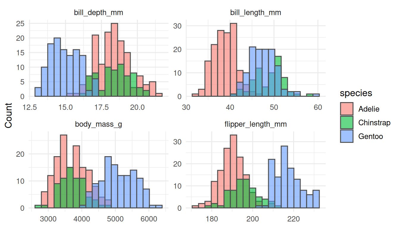

All four continuous variables are approximately symmetric within species, so mean (SD) is defensible. If a variable were skewed, we would switch to median (IQR).

t1 <- dat |>
  select(species, sex, bill_length_mm, bill_depth_mm,
         flipper_length_mm, body_mass_g) |>
  tbl_summary(
    by = species,
    statistic = list(
      all_continuous() ~ "{mean} ({sd})",
      all_categorical() ~ "{n} ({p}%)"
    ),
    digits = all_continuous() ~ 1,
    label = list(
      bill_length_mm    ~ "Bill length (mm)",
      bill_depth_mm     ~ "Bill depth (mm)",
      flipper_length_mm ~ "Flipper length (mm)",
      body_mass_g       ~ "Body mass (g)",
      sex               ~ "Sex"
    )
  ) |>
  add_overall() |>
  add_p()
t1

Characteristic	Overall N = 333¹	Adelie N = 146¹	Chinstrap N = 68¹	Gentoo N = 119¹	p-value²
Sex					>0.9
female	165 (50%)	73 (50%)	34 (50%)	58 (49%)
male	168 (50%)	73 (50%)	34 (50%)	61 (51%)
Bill length (mm)	44.0 (5.5)	38.8 (2.7)	48.8 (3.3)	47.6 (3.1)	<0.001
Bill depth (mm)	17.2 (2.0)	18.3 (1.2)	18.4 (1.1)	15.0 (1.0)	<0.001
Flipper length (mm)	201.0 (14.0)	190.1 (6.5)	195.8 (7.1)	217.2 (6.6)	<0.001
Body mass (g)	4,207.1 (805.2)	3,706.2 (458.6)	3,733.1 (384.3)	5,092.4 (501.5)	<0.001
¹ n (%); Mean (SD)
² Pearson’s Chi-squared test; Kruskal-Wallis rank sum test

add_p() will run a t-test or ANOVA on continuous variables and a chi-square or Fisher’s exact test on categorical, with sensible defaults for sample size.

4. Check

Validate the gtsummary output against a hand computation.

dat |>
  group_by(species) |>
  summarise(
    n = n(),
    mean_mass = mean(body_mass_g),
    sd_mass   = sd(body_mass_g),
    .groups = "drop"
  )

# A tibble: 3 × 4
  species       n mean_mass sd_mass
  <fct>     <int>     <dbl>   <dbl>
1 Adelie      146     3706.    459.
2 Chinstrap    68     3733.    384.
3 Gentoo      119     5092.    501.

The group means and standard deviations must match the numbers in the body-mass row of the Table 1.

5. Report

Table 1 describes 333 penguins from three species in the Palmer Archipelago. Body mass was highest in Gentoo (5092 ± 501 g) and lower in Adelie and Chinstrap. All four continuous variables were approximately symmetric within species and are summarised as mean (SD); sex was approximately balanced within each species.

Table 1 is not a tool for hypothesis testing. The p-values in the rightmost column describe the data, not the biology. A statistically-significant difference between arms at baseline in a randomised trial is, by construction, a chance finding.

Stress the distinction between Table 1 as description and Table 2 as inference. The audience will carry the habit into their own writing.

Common pitfalls

Reporting a mean for a skewed variable.
Using Table 1 as a place to “prove balance” with p-values in a randomised trial.
Suppressing the missing-data row. Always report it.
Forgetting that tbl_summary drops NAs by default; check the count at the bottom of each column.

Session info

sessionInfo()

R version 4.4.1 (2024-06-14)
Platform: x86_64-pc-linux-gnu
Running under: Ubuntu 24.04.4 LTS

Matrix products: default
BLAS:   /usr/lib/x86_64-linux-gnu/openblas-pthread/libblas.so.3 
LAPACK: /usr/lib/x86_64-linux-gnu/openblas-pthread/libopenblasp-r0.3.26.so;  LAPACK version 3.12.0

locale:
 [1] LC_CTYPE=C.UTF-8       LC_NUMERIC=C           LC_TIME=C.UTF-8       
 [4] LC_COLLATE=C.UTF-8     LC_MONETARY=C.UTF-8    LC_MESSAGES=C.UTF-8   
 [7] LC_PAPER=C.UTF-8       LC_NAME=C              LC_ADDRESS=C          
[10] LC_TELEPHONE=C         LC_MEASUREMENT=C.UTF-8 LC_IDENTIFICATION=C   

time zone: UTC
tzcode source: system (glibc)

attached base packages:
[1] stats     graphics  grDevices utils     datasets  methods   base     

other attached packages:
 [1] gtsummary_2.5.0      palmerpenguins_0.1.1 lubridate_1.9.5     
 [4] forcats_1.0.1        stringr_1.6.0        dplyr_1.2.1         
 [7] purrr_1.2.2          readr_2.2.0          tidyr_1.3.2         
[10] tibble_3.3.1         ggplot2_4.0.3        tidyverse_2.0.0     

loaded via a namespace (and not attached):
 [1] gt_1.3.0           utf8_1.2.6         sass_0.4.10        generics_0.1.4    
 [5] xml2_1.5.2         stringi_1.8.7      hms_1.1.4          digest_0.6.39     
 [9] magrittr_2.0.5     evaluate_1.0.5     grid_4.4.1         timechange_0.4.0  
[13] RColorBrewer_1.1-3 cards_0.7.1        fastmap_1.2.0      jsonlite_2.0.0    
[17] cardx_0.3.2        backports_1.5.1    scales_1.4.0       cli_3.6.6         
[21] rlang_1.2.0        litedown_0.9       commonmark_2.0.0   base64enc_0.1-6   
[25] withr_3.0.2        yaml_2.3.12        otel_0.2.0         tools_4.4.1       
[29] tzdb_0.5.0         broom_1.0.12       vctrs_0.7.3        R6_2.6.1          
[33] lifecycle_1.0.5    fs_2.1.0           htmlwidgets_1.6.4  pkgconfig_2.0.3   
[37] pillar_1.11.1      gtable_0.3.6       glue_1.8.1         xfun_0.57         
[41] tidyselect_1.2.1   knitr_1.51         farver_2.1.2       htmltools_0.5.9   
[45] rmarkdown_2.31     labeling_0.4.3     compiler_4.4.1     S7_0.2.2          
[49] markdown_2.0

Learning objectives

Prerequisites

Background

Setup

1. Goal

2. Approach

3. Execution

4. Check

5. Report

Common pitfalls

Further reading

Session info

Related labs