library(tidyverse)
library(broom)
set.seed(42)
theme_set(theme_minimal(base_size = 12))Week 1, Session 3 — Multiple regression: confounding, interaction, centring
Course 2 — #courses
Note
Inference labs use the five-step template: Hypothesis → Visualise → Assumptions → Conduct → Conclude.
Learning objectives
- Distinguish confounding from mediation and from effect modification.
- Read a multiple regression coefficient as an adjusted effect.
- Centre predictors before fitting interactions and explain why.
Prerequisites
Sessions 1 and 2 of this week.
Background
Multiple regression is the standard way to estimate the effect of one predictor while holding others constant. The word holding is doing a lot of work: the adjusted coefficient is the effect conditional on the other variables in the model, not the effect one would observe in a new study that intervened on them. Confounding, mediation, and collider bias all pivot on which covariates are in the model. The statistics textbook cannot answer that question; the subject-matter science must.
Interactions complicate this picture. When two predictors interact, the effect of one depends on the level of the other, and the main-effect coefficient becomes the effect when the interacting variable is zero. Centring continuous predictors before fitting an interaction restores a readable interpretation: the main effect becomes the effect at the sample mean of the other variable, which is usually what the reader wants.
Collinearity and scale are often discussed together. Centring does not reduce real collinearity between X and Z, but it does reduce the algebraic collinearity between X and X·Z that otherwise makes the coefficients hard to interpret and inflates their standard errors.
Setup
1. Hypothesis
Simulate a scenario in which a confounder masks the effect of interest, then add an interaction to show effect modification.
2. Visualise
n <- 300
age <- rnorm(n, 55, 10)
# smoker more common among older people in this simulation (confounding)
smoker <- rbinom(n, 1, plogis(-3 + 0.05 * age))
# outcome depends on both; smoker effect is stronger at older ages (interaction)
y <- 120 + 0.6 * age + 5 * smoker + 0.2 * smoker * (age - mean(age)) +
  rnorm(n, 0, 8)
dat <- tibble(age, smoker = factor(smoker, labels = c("no", "yes")), y)

ggplot(dat, aes(age, y, colour = smoker)) +
  geom_point(alpha = 0.6) +
  geom_smooth(method = "lm", se = FALSE) +
  labs(x = "Age (years)", y = "Outcome", colour = "Smoker")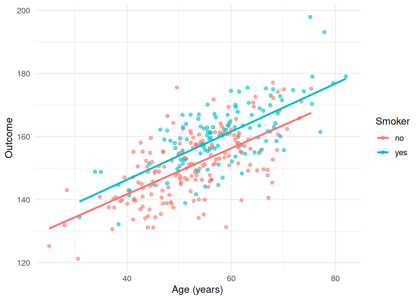
Both lines climb with age; the smoker line sits higher and may slope more steeply.
3. Assumptions
The usual linear-model assumptions, plus an implicit assumption that all relevant confounders are in the model.
fit_full <- lm(y ~ age * smoker, data = dat)
par(mfrow = c(2, 2))
plot(fit_full)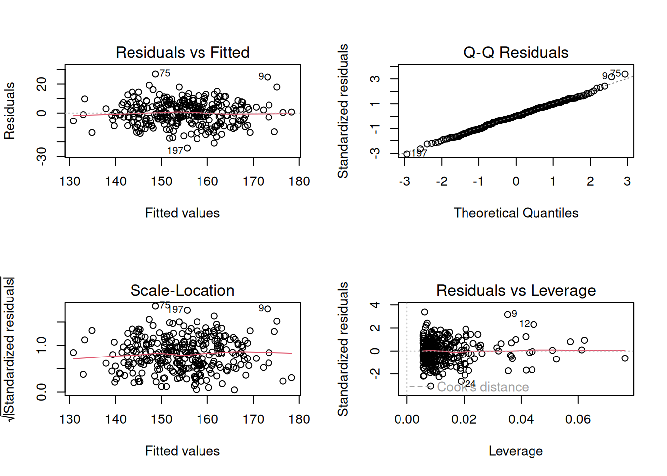
par(mfrow = c(1, 1))4. Conduct
Crude smoker effect, then adjusted for age, then with interaction:
crude    <- lm(y ~ smoker, data = dat)
adjusted <- lm(y ~ smoker + age, data = dat)
inter    <- lm(y ~ smoker * age, data = dat)

bind_rows(
  tidy(crude, conf.int = TRUE) |> mutate(model = "crude"),
  tidy(adjusted, conf.int = TRUE) |> mutate(model = "adjusted"),
  tidy(inter, conf.int = TRUE) |> mutate(model = "interaction")
) |>
  filter(term != "(Intercept)") |>
  select(model, term, estimate, conf.low, conf.high, p.value)
# A tibble: 6 × 6
model term estimate conf.low conf.high p.value
<chr> <chr> <dbl> <dbl> <dbl> <dbl>
1 crude smokeryes 9.25 6.79 11.7 1.29e-12
2 adjusted smokeryes 5.14 3.22 7.05 2.49e- 7
3 adjusted age 0.742 0.647 0.838 2.53e-39
4 interaction smokeryes 3.29 -7.77 14.4 5.58e- 1
5 interaction age 0.729 0.605 0.853 7.05e-26
6 interaction smokeryes:age 0.0330 -0.162 0.228 7.39e- 1Now with centred age, which makes the smokeryes coefficient the smoker effect at mean age:
dat_c <- dat |> mutate(age_c = age - mean(age))
inter_c <- lm(y ~ smoker * age_c, data = dat_c)
tidy(inter_c, conf.int = TRUE)
# A tibble: 4 × 7
term estimate std.error statistic p.value conf.low conf.high
<chr> <dbl> <dbl> <dbl> <dbl> <dbl> <dbl>
1 (Intercept) 152. 0.616 247. 0 151. 154.
2 smokeryes 5.10 0.980 5.21 3.57e- 7 3.17 7.03
3 age_c 0.729 0.0629 11.6 7.05e-26 0.605 0.853
4 smokeryes:age_c 0.0330 0.0992 0.333 7.39e- 1 -0.162 0.2285. Concluding statement
After adjusting for age, the estimated smoker-effect at the sample mean age was 5.1 units (95% CI: 3.2 to 7), with evidence of effect modification by age (interaction coefficient 0.03).
The point here is that adjusted is not a synonym for causal, and that centring is a small habit with a large readability payoff.
Common pitfalls
- Reading an adjusted coefficient as a population-level causal effect without thinking about what the adjustment set represents.
- Fitting an interaction without centring and then trying to interpret the main effects.
- Dropping covariates that look non-significant one at a time.
Further reading
- Greenland S (1998), Confounding and collapsibility in causal inference.
- VanderWeele TJ. Explanation in Causal Inference.
- Fox J. Applied Regression Analysis and Generalized Linear Models.
Session info
sessionInfo()R version 4.5.2 (2025-10-31 ucrt)
Platform: x86_64-w64-mingw32/x64
Running under: Windows 11 x64 (build 26200)
Matrix products: default
LAPACK version 3.12.1
locale:
[1] LC_COLLATE=English_Germany.utf8 LC_CTYPE=English_Germany.utf8
[3] LC_MONETARY=English_Germany.utf8 LC_NUMERIC=C
[5] LC_TIME=English_Germany.utf8
time zone: Europe/Berlin
tzcode source: internal
attached base packages:
[1] stats graphics grDevices utils datasets methods base
other attached packages:
[1] broom_1.0.12 lubridate_1.9.5 forcats_1.0.1 stringr_1.6.0
[5] dplyr_1.2.1 purrr_1.2.2 readr_2.2.0 tidyr_1.3.2
[9] tibble_3.3.1 ggplot2_4.0.3 tidyverse_2.0.0
loaded via a namespace (and not attached):
[1] Matrix_1.7-5 gtable_0.3.6 jsonlite_2.0.0 compiler_4.5.2
[5] tidyselect_1.2.1 splines_4.5.2 scales_1.4.0 yaml_2.3.12
[9] fastmap_1.2.0 lattice_0.22-9 R6_2.6.1 labeling_0.4.3
[13] generics_0.1.4 knitr_1.51 backports_1.5.1 htmlwidgets_1.6.4
[17] pillar_1.11.1 RColorBrewer_1.1-3 tzdb_0.5.0 rlang_1.2.0
[21] utf8_1.2.6 stringi_1.8.7 xfun_0.57 S7_0.2.2
[25] otel_0.2.0 timechange_0.4.0 cli_3.6.6 mgcv_1.9-4
[29] withr_3.0.2 magrittr_2.0.4 digest_0.6.39 grid_4.5.2
[33] hms_1.1.4 nlme_3.1-169 lifecycle_1.0.5 vctrs_0.7.3
[37] evaluate_1.0.5 glue_1.8.1 farver_2.1.2 rmarkdown_2.31
[41] tools_4.5.2 pkgconfig_2.0.3 htmltools_0.5.9