Week 1, Session 1 — Correlation vs regression; Model-I/II regression

Course 2 — #courses

Author

R. Heller

Note

Inference labs use the five-step template: Hypothesis → Visualise → Assumptions → Conduct → Conclude.

Learning objectives

Distinguish correlation from regression and say when each is appropriate.
Fit Model-I (OLS) and Model-II (major-axis / SMA) lines and interpret the difference.
Report an association with a slope, interval, and p-value rather than with a correlation alone.

Prerequisites

Course 1, or equivalent exposure to hypothesis testing and basic R.

Background

Correlation and regression answer related but different questions. Correlation asks how tightly do two variables track each other? and is symmetric in X and Y. Regression asks how does the mean of Y change with X? and treats the two axes asymmetrically: X is assumed to be measured without error and Y is modelled. This asymmetry matters for prediction (which needs a regression line) and for comparing slopes across groups (which also needs regression), but it becomes problematic when both variables carry measurement error and neither can be declared the predictor.

Model-II regression — of which the standardised major axis (SMA) and reduced major axis are the common flavours — was developed for exactly this case. When both X and Y are measured with error, ordinary least squares (OLS) is biased toward zero, because it attributes all residual variation to Y. Model-II methods acknowledge error in both directions and give a less biased estimate of the true functional relationship. The price is a weaker theoretical grounding for inference and the need to report the method used.

Model-II regression has a respectable history in allometry and in method-comparison studies, where the instruments on both axes are imperfect. In a clinical lab context you will often see Deming regression for comparing two assays; SMA and Deming are close cousins under reasonable assumptions. The choice should follow the science: is X a fixed, controlled input, or a noisy measurement of something?

Setup

library(tidyverse)
library(broom)
set.seed(42)
theme_set(theme_minimal(base_size = 12))

1. Hypothesis

We will simulate two noisy measurements of the same underlying quantity — say, body size measured by two instruments — and ask how OLS and SMA differ.

Null hypothesis: the two measurements are uncorrelated. Working alternative: they are positively associated, with a slope near 1 if the instruments agree.

2. Visualise

n <- 200
true_size <- rnorm(n, mean = 50, sd = 10)
x <- true_size + rnorm(n, 0, 3)
y <- true_size + rnorm(n, 0, 3)
dat <- tibble(x, y)

ggplot(dat, aes(x, y)) +
  geom_point(alpha = 0.6, colour = "grey30") +
  labs(x = "Instrument 1", y = "Instrument 2")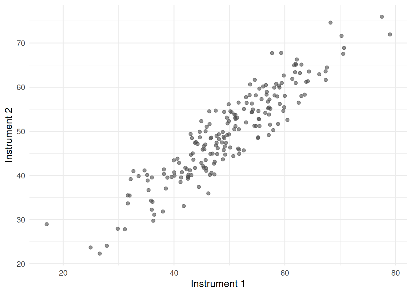

A cloud of points that climbs from lower-left to upper-right. Both instruments carry error, so neither deserves to be called the truth.

3. Assumptions

OLS assumes X is measured without error and residuals in Y are approximately normal with constant variance. SMA assumes errors in both variables are comparable in scale. Both assume linearity.

fit_ols <- lm(y ~ x, data = dat)
par(mfrow = c(1, 2))
plot(fit_ols, which = c(1, 2))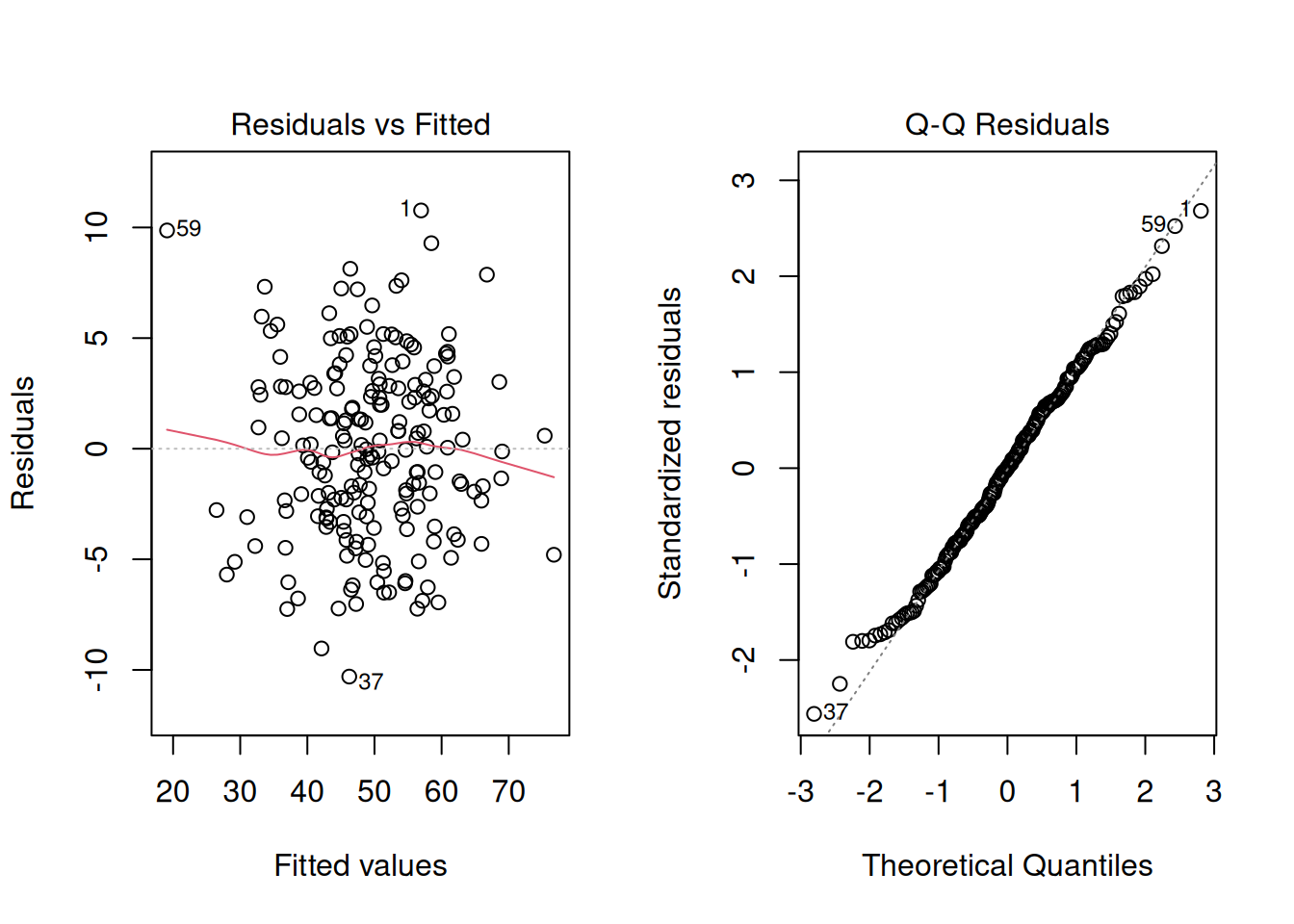

par(mfrow = c(1, 1))

Residuals look patternless; the QQ plot is close to the diagonal. The OLS diagnostics are fine; they just do not capture the fact that X is also noisy.

4. Conduct

cor.test(dat$x, dat$y)


    Pearson's product-moment correlation

data:  dat$x and dat$y
t = 32.297, df = 198, p-value < 2.2e-16
alternative hypothesis: true correlation is not equal to 0
95 percent confidence interval:
 0.8914103 0.9364059
sample estimates:
      cor 
0.9167697

fit_ols <- lm(y ~ x, data = dat)
tidy(fit_ols, conf.int = TRUE)

# A tibble: 2 × 7
  term        estimate std.error statistic  p.value conf.low conf.high
  <chr>          <dbl>     <dbl>     <dbl>    <dbl>    <dbl>     <dbl>
1 (Intercept)    3.27     1.46        2.24 2.62e- 2    0.393     6.15 
2 x              0.930    0.0288     32.3  7.46e-81    0.873     0.987

Now a hand-coded SMA slope. The SMA slope is the ratio of standard deviations, signed by the correlation:

sma_slope <- function(x, y) sign(cor(x, y)) * sd(y) / sd(x)
sma_intercept <- function(x, y) mean(y) - sma_slope(x, y) * mean(x)

b_sma <- sma_slope(dat$x, dat$y)
a_sma <- sma_intercept(dat$x, dat$y)
b_ols <- coef(fit_ols)[2]

c(ols_slope = unname(b_ols), sma_slope = b_sma)

ols_slope sma_slope 
0.9300472 1.0144830

ggplot(dat, aes(x, y)) +
  geom_point(alpha = 0.5, colour = "grey40") +
  geom_abline(intercept = coef(fit_ols)[1], slope = b_ols,
              colour = "steelblue", linewidth = 0.9) +
  geom_abline(intercept = a_sma, slope = b_sma,
              colour = "firebrick", linewidth = 0.9, linetype = 2) +
  labs(x = "Instrument 1", y = "Instrument 2",
       title = "OLS (blue) vs SMA (red)")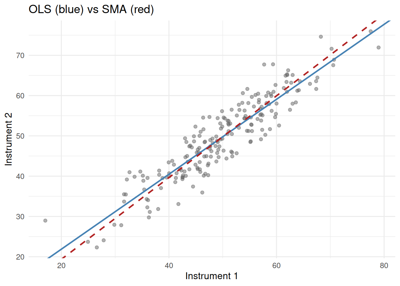

The SMA slope is closer to 1. OLS is attenuated because it treats X as fixed when it is not.

5. Concluding statement

In simulated data (n = 200), instrument 2 increased with instrument 1 (Pearson r = 0.92; OLS slope 0.93; SMA slope 1.01). Because both instruments carry measurement error, we report the SMA slope as the functional relationship and note the OLS slope for comparison.

Emphasise that the question — prediction vs functional relationship — drives the choice, not a preference for one method.

Common pitfalls

Reporting a correlation when a slope is what the reader needs.
Using OLS to compare two noisy measurements and concluding the slope differs from 1 when the attenuation is an artefact.
Forgetting that r has no units and therefore cannot substitute for an effect size on the measurement scale.

Session info

sessionInfo()

R version 4.4.1 (2024-06-14)
Platform: x86_64-pc-linux-gnu
Running under: Ubuntu 24.04.4 LTS

Matrix products: default
BLAS:   /usr/lib/x86_64-linux-gnu/openblas-pthread/libblas.so.3 
LAPACK: /usr/lib/x86_64-linux-gnu/openblas-pthread/libopenblasp-r0.3.26.so;  LAPACK version 3.12.0

locale:
 [1] LC_CTYPE=C.UTF-8       LC_NUMERIC=C           LC_TIME=C.UTF-8       
 [4] LC_COLLATE=C.UTF-8     LC_MONETARY=C.UTF-8    LC_MESSAGES=C.UTF-8   
 [7] LC_PAPER=C.UTF-8       LC_NAME=C              LC_ADDRESS=C          
[10] LC_TELEPHONE=C         LC_MEASUREMENT=C.UTF-8 LC_IDENTIFICATION=C   

time zone: UTC
tzcode source: system (glibc)

attached base packages:
[1] stats     graphics  grDevices utils     datasets  methods   base     

other attached packages:
 [1] broom_1.0.12    lubridate_1.9.5 forcats_1.0.1   stringr_1.6.0  
 [5] dplyr_1.2.1     purrr_1.2.2     readr_2.2.0     tidyr_1.3.2    
 [9] tibble_3.3.1    ggplot2_4.0.3   tidyverse_2.0.0

loaded via a namespace (and not attached):
 [1] gtable_0.3.6       jsonlite_2.0.0     compiler_4.4.1     tidyselect_1.2.1  
 [5] scales_1.4.0       yaml_2.3.12        fastmap_1.2.0      R6_2.6.1          
 [9] labeling_0.4.3     generics_0.1.4     knitr_1.51         backports_1.5.1   
[13] htmlwidgets_1.6.4  pillar_1.11.1      RColorBrewer_1.1-3 tzdb_0.5.0        
[17] rlang_1.2.0        utf8_1.2.6         stringi_1.8.7      xfun_0.57         
[21] S7_0.2.2           otel_0.2.0         timechange_0.4.0   cli_3.6.6         
[25] withr_3.0.2        magrittr_2.0.5     digest_0.6.39      grid_4.4.1        
[29] hms_1.1.4          lifecycle_1.0.5    vctrs_0.7.3        evaluate_1.0.5    
[33] glue_1.8.1         farver_2.1.2       rmarkdown_2.31     tools_4.4.1       
[37] pkgconfig_2.0.3    htmltools_0.5.9

Learning objectives

Prerequisites

Background

Setup

1. Hypothesis

2. Visualise

3. Assumptions

4. Conduct

5. Concluding statement

Common pitfalls

Further reading

Session info

Related labs