Week 2, Session 2 — Two-way / factorial ANOVA with interaction

Course 2 — #courses

Author

R. Heller

Note

Inference labs use the five-step template: Hypothesis → Visualise → Assumptions → Conduct → Conclude.

Learning objectives

Fit a two-factor ANOVA and distinguish main effects from interactions.
Visualise an interaction with emmip() and read the picture before the table.
Report a factorial analysis in the correct order: interaction first, then conditional main effects.

Prerequisites

Session 1 of this week.

Background

A factorial design crosses two (or more) categorical factors. The two-way ANOVA decomposes variability into main effects and the interaction between factors. If the interaction is negligible, main effects can be reported as averages across levels of the other factor; if not, the main-effect table is misleading and conditional (simple) effects must be reported instead.

The canonical small dataset is ToothGrowth, which crosses dose of vitamin C with delivery method (orange juice vs ascorbic acid). It is a complete factorial and nicely balanced, which means the classification of variance into Type-I, Type-II, and Type-III sums of squares does not matter. With unbalanced designs it does, and Type-III via car::Anova with contrasts set to contr.sum is the usual safe choice.

Plotting the interaction is almost always the right first step. An interaction plot that shows parallel lines agrees with an insignificant interaction term; crossed lines signal an interaction; lines with different slopes signal a quantitative interaction.

Setup

library(tidyverse)
library(broom)
library(car)
library(emmeans)
set.seed(42)
theme_set(theme_minimal(base_size = 12))

1. Hypothesis

Does delivery method alter the effect of dose on tooth length?

Null: no interaction between supp and dose. Alternative: the dose effect differs by supp.

2. Visualise

tg <- ToothGrowth |> mutate(dose = factor(dose))

ggplot(tg, aes(dose, len, colour = supp, group = supp)) +
  stat_summary(fun = mean, geom = "point", size = 3) +
  stat_summary(fun = mean, geom = "line") +
  stat_summary(fun.data = mean_cl_normal, geom = "errorbar", width = 0.1) +
  labs(x = "Dose (mg/day)", y = "Tooth length", colour = "Supp")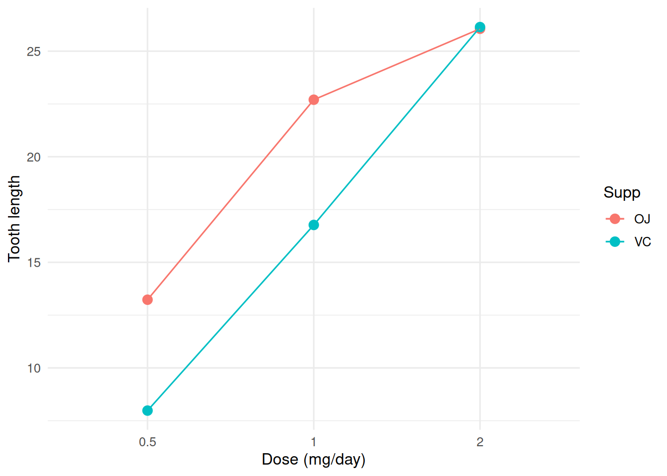

3. Assumptions

fit <- aov(len ~ supp * dose, data = tg)
par(mfrow = c(2, 2))
plot(fit)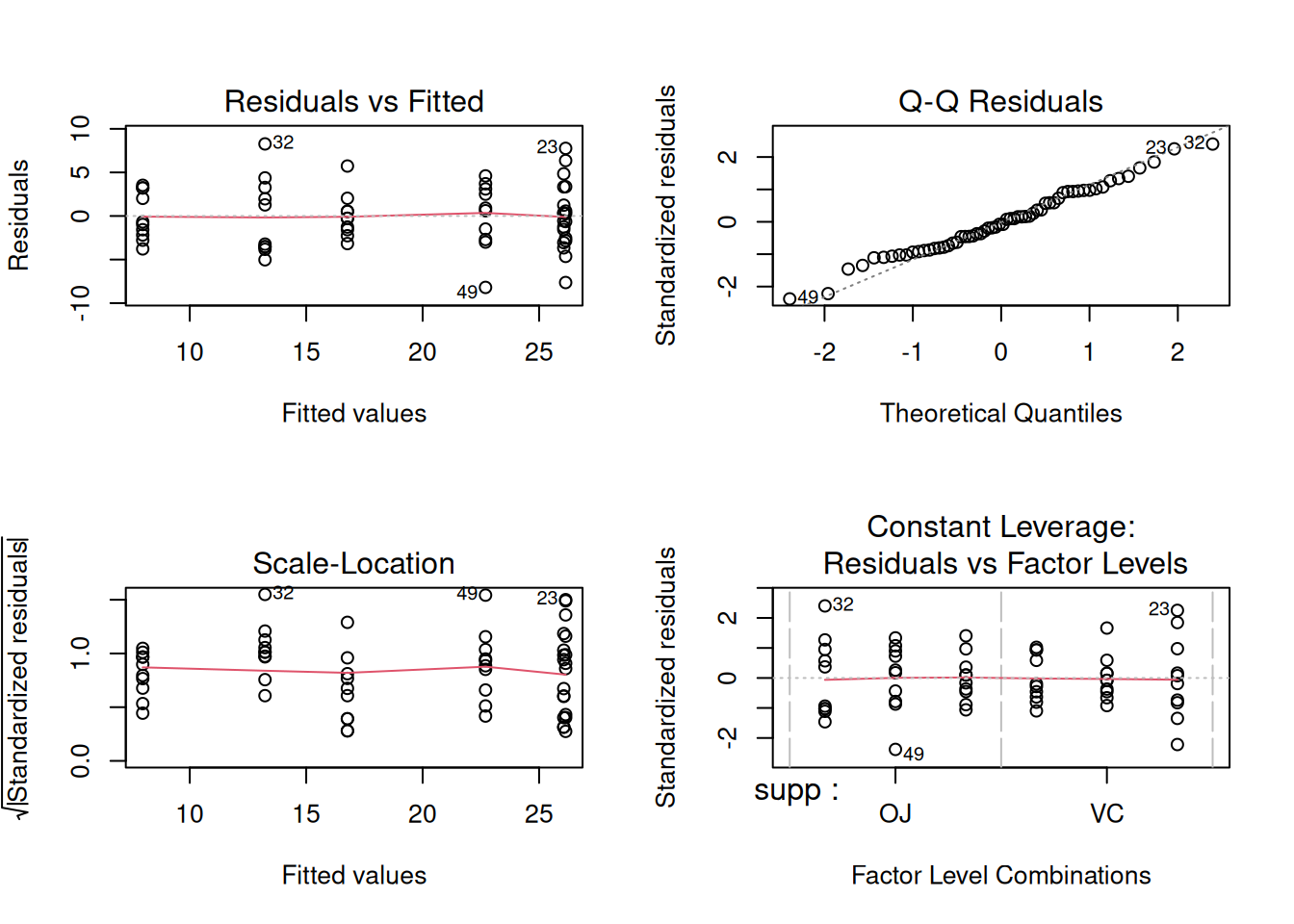

par(mfrow = c(1, 1))

4. Conduct

# Type-II sums of squares for a balanced design
Anova(lm(len ~ supp * dose, data = tg), type = 2)

Anova Table (Type II tests)

Response: len
           Sum Sq Df F value    Pr(>F)    
supp       205.35  1  15.572 0.0002312 ***
dose      2426.43  2  92.000 < 2.2e-16 ***
supp:dose  108.32  2   4.107 0.0218603 *  
Residuals  712.11 54                      
---
Signif. codes:  0 '***' 0.001 '**' 0.01 '*' 0.05 '.' 0.1 ' ' 1

emm <- emmeans(fit, ~ supp | dose)
pairs(emm)

dose = 0.5:
 contrast estimate   SE df t.ratio p.value
 OJ - VC      5.25 1.62 54   3.233  0.0021

dose = 1:
 contrast estimate   SE df t.ratio p.value
 OJ - VC      5.93 1.62 54   3.651  0.0006

dose = 2:
 contrast estimate   SE df t.ratio p.value
 OJ - VC     -0.08 1.62 54  -0.049  0.9609

emmip(fit, supp ~ dose, CIs = TRUE)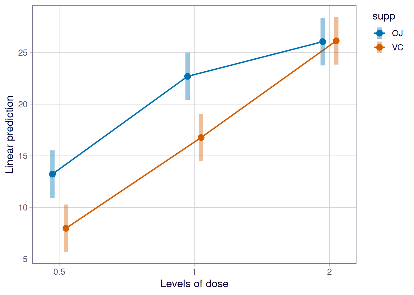

5. Concluding statement

Tooth length responded to dose (large main effect) and to supplement (smaller main effect), with evidence of an interaction (see ANOVA table). The difference between orange juice and ascorbic acid was largest at the lowest dose and negligible at the highest.

Use the interaction plot to justify the order of the report: when the lines are not parallel, the main-effect column in the ANOVA table is only a summary, not the headline.

Common pitfalls

Reporting main effects without first checking the interaction.
Using Type-III sums of squares with default treatment contrasts in unbalanced designs; the output depends on the contrast coding.
Ignoring unequal cell sizes when reading an ANOVA table.

Session info

sessionInfo()

R version 4.4.1 (2024-06-14)
Platform: x86_64-pc-linux-gnu
Running under: Ubuntu 24.04.4 LTS

Matrix products: default
BLAS:   /usr/lib/x86_64-linux-gnu/openblas-pthread/libblas.so.3 
LAPACK: /usr/lib/x86_64-linux-gnu/openblas-pthread/libopenblasp-r0.3.26.so;  LAPACK version 3.12.0

locale:
 [1] LC_CTYPE=C.UTF-8       LC_NUMERIC=C           LC_TIME=C.UTF-8       
 [4] LC_COLLATE=C.UTF-8     LC_MONETARY=C.UTF-8    LC_MESSAGES=C.UTF-8   
 [7] LC_PAPER=C.UTF-8       LC_NAME=C              LC_ADDRESS=C          
[10] LC_TELEPHONE=C         LC_MEASUREMENT=C.UTF-8 LC_IDENTIFICATION=C   

time zone: UTC
tzcode source: system (glibc)

attached base packages:
[1] stats     graphics  grDevices utils     datasets  methods   base     

other attached packages:
 [1] emmeans_2.0.3   car_3.1-5       carData_3.0-6   broom_1.0.12   
 [5] lubridate_1.9.5 forcats_1.0.1   stringr_1.6.0   dplyr_1.2.1    
 [9] purrr_1.2.2     readr_2.2.0     tidyr_1.3.2     tibble_3.3.1   
[13] ggplot2_4.0.3   tidyverse_2.0.0

loaded via a namespace (and not attached):
 [1] generics_0.1.4     stringi_1.8.7      lattice_0.22-6     hms_1.1.4         
 [5] digest_0.6.39      magrittr_2.0.5     evaluate_1.0.5     grid_4.4.1        
 [9] timechange_0.4.0   estimability_1.5.1 RColorBrewer_1.1-3 mvtnorm_1.3-7     
[13] fastmap_1.2.0      jsonlite_2.0.0     backports_1.5.1    Formula_1.2-5     
[17] scales_1.4.0       abind_1.4-8        cli_3.6.6          rlang_1.2.0       
[21] withr_3.0.2        yaml_2.3.12        otel_0.2.0         tools_4.4.1       
[25] tzdb_0.5.0         coda_0.19-4.1      vctrs_0.7.3        R6_2.6.1          
[29] lifecycle_1.0.5    htmlwidgets_1.6.4  pkgconfig_2.0.3    pillar_1.11.1     
[33] gtable_0.3.6       glue_1.8.1         xfun_0.57          tidyselect_1.2.1  
[37] knitr_1.51         xtable_1.8-8       farver_2.1.2       htmltools_0.5.9   
[41] labeling_0.4.3     rmarkdown_2.31     compiler_4.4.1     S7_0.2.2

Learning objectives

Prerequisites

Background

Setup

1. Hypothesis

2. Visualise

3. Assumptions

4. Conduct

5. Concluding statement

Common pitfalls

Further reading

Session info

Related labs