library(tidyverse)
library(mice)
set.seed(42)
theme_set(theme_minimal(base_size = 12))Week 2, Session 2 — Multiple imputation with mice
Course 3 — #courses
Note
Inference lab using the five-step template: Hypothesis → Visualise → Assumptions → Conduct → Conclude.
Learning objectives
- Run multiple imputation by chained equations with
mice. - Diagnose convergence with trace and density plots.
- Pool regression coefficients across imputations using Rubin’s rules.
Prerequisites
Session 1 of this week (MCAR/MAR/MNAR).
Background
Multiple imputation (MI) replaces each missing value with several plausible values drawn from a predictive distribution, producing m completed datasets. Each completed dataset is analysed separately; the results are pooled using Rubin’s rules so that the standard errors reflect both the within-imputation uncertainty (ordinary sampling variance) and the between-imputation uncertainty (the variance of the imputations themselves).
mice implements MI by chained equations: for each incomplete variable, it fits a conditional model given the others and draws imputations from the posterior predictive distribution of that model. The procedure iterates until the imputations stabilise. The standard diagnostics are trace plots (should mix and not drift) and density plots comparing observed and imputed values (should overlap but need not match exactly).
The inclusion of the outcome in the imputation model is not optional. Omitting it biases the imputations toward the null and attenuates the estimated effect in the pooled analysis.
Setup
1. Hypothesis
In the mice::nhanes teaching dataset, the cholesterol outcome (chl) is related to age and BMI (bmi). We will estimate that relationship under MI.
2. Visualise
data(nhanes, package = "mice")
md.pattern(nhanes, plot = FALSE)
age hyp bmi chl
13 1 1 1 1 0
3 1 1 1 0 1
1 1 1 0 1 1
1 1 0 0 1 2
7 1 0 0 0 3
0 8 9 10 27nhanes |>
mutate(missing_chl = is.na(chl)) |>
ggplot(aes(bmi, chl, colour = missing_chl)) +
geom_point(size = 2) +
labs(x = "BMI", y = "Cholesterol", colour = "chl missing?")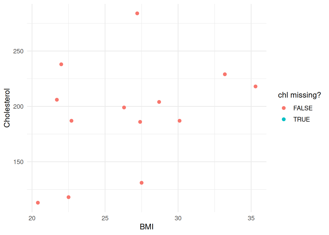
3. Assumptions
MAR conditional on the variables in the imputation model; a compatible imputation model (predictive mean matching by default); enough imputations (here m = 10) to stabilise the pooled standard errors.
4. Conduct
imp <- mice(nhanes, m = 10, method = "pmm",
            printFlag = FALSE, seed = 42)
imp
Class: mids
Number of multiple imputations: 10
Imputation methods:
age bmi hyp chl
"" "pmm" "pmm" "pmm"
PredictorMatrix:
age bmi hyp chl
age 0 1 1 1
bmi 1 0 1 1
hyp 1 1 0 1
chl 1 1 1 0plot(imp)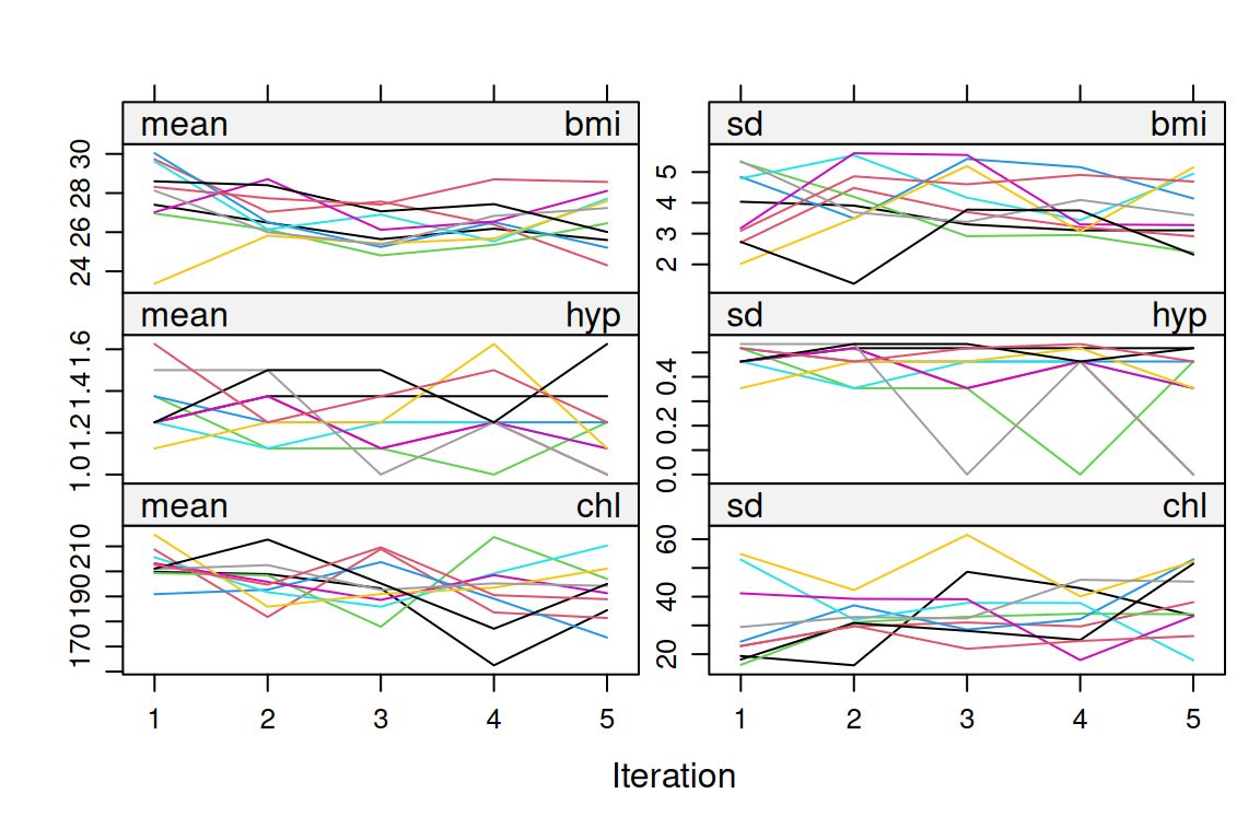
densityplot(imp)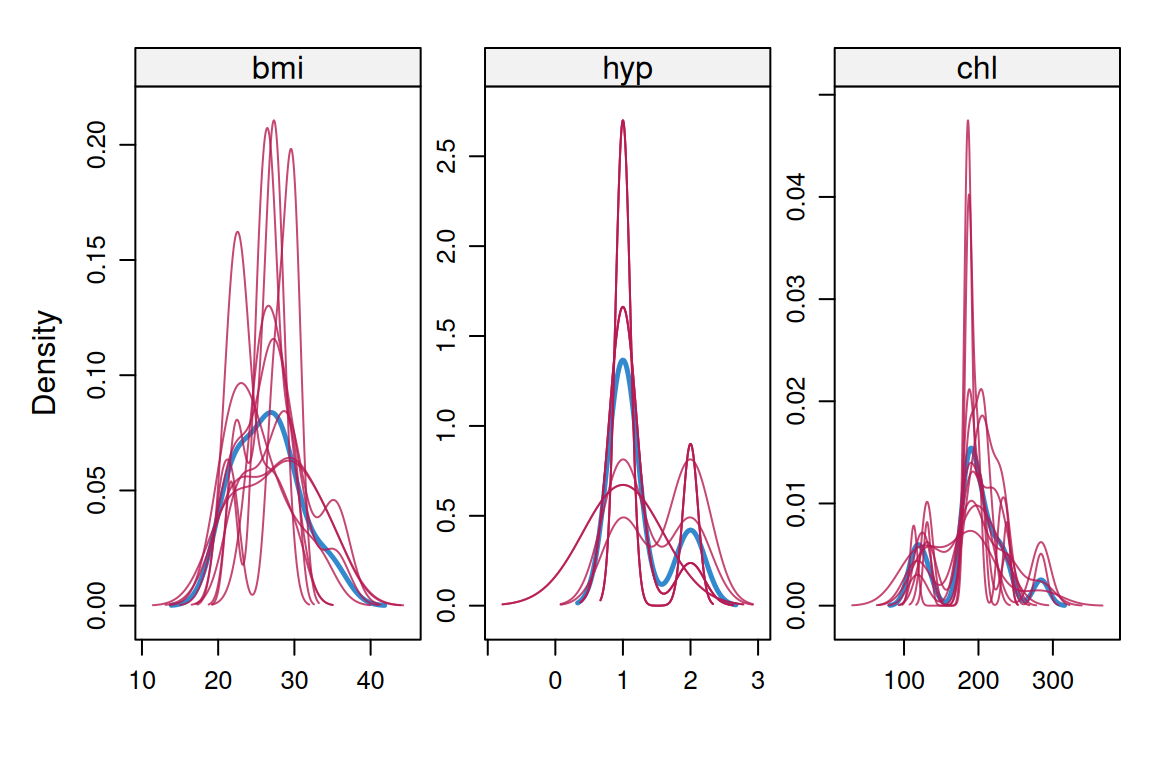
fit   <- with(imp, lm(chl ~ age + bmi))
pooled <- pool(fit)
summary(pooled, conf.int = TRUE)
term estimate std.error statistic df p.value 2.5 %
1 (Intercept) -22.553452 60.422948 -0.3732597 17.319419 0.71348446 -149.855865
2 age 35.321205 11.255699 3.1380730 9.947218 0.01061075 10.223895
3 bmi 5.711016 2.036136 2.8048302 14.980225 0.01334229 1.370596
97.5 % conf.low conf.high
1 104.74896 -149.855865 104.74896
2 60.41852 10.223895 60.41852
3 10.05144 1.370596 10.051445. Concluding statement
Multiple imputation of the
nhanesdataset (m = 10, predictive mean matching) gave a pooled coefficient for BMI on cholesterol of 5.71 (see pooled table above), with standard errors reflecting both within- and between-imputation uncertainty through Rubin’s rules.
Students should leave this session able to say out loud that “MI accounts for missing-data uncertainty” does not mean “MI fixes MNAR”. It does not.
Common pitfalls
- Imputing the outcome separately from the covariates with incompatible models.
- Using m = 5 when the fraction of missing information is high.
- Pooling means or SDs by hand instead of
pool(). - Dropping the outcome from the imputation model because it “feels like cheating”.
Further reading
- van Buuren S, Groothuis-Oudshoorn K (2011), mice: Multivariate Imputation by Chained Equations in R.
- van Buuren S (2018), Flexible Imputation of Missing Data, ch. 4–6.
- White IR, Royston P, Wood AM (2011), Multiple imputation using chained equations: issues and guidance for practice.
Session info
sessionInfo()R version 4.5.2 (2025-10-31 ucrt)
Platform: x86_64-w64-mingw32/x64
Running under: Windows 11 x64 (build 26200)
Matrix products: default
LAPACK version 3.12.1
locale:
[1] LC_COLLATE=English_Germany.utf8 LC_CTYPE=English_Germany.utf8
[3] LC_MONETARY=English_Germany.utf8 LC_NUMERIC=C
[5] LC_TIME=English_Germany.utf8
time zone: Europe/Berlin
tzcode source: internal
attached base packages:
[1] stats graphics grDevices utils datasets methods base
other attached packages:
[1] mice_3.19.0 lubridate_1.9.5 forcats_1.0.1 stringr_1.6.0
[5] dplyr_1.2.1 purrr_1.2.2 readr_2.2.0 tidyr_1.3.2
[9] tibble_3.3.1 ggplot2_4.0.3 tidyverse_2.0.0
loaded via a namespace (and not attached):
[1] gtable_0.3.6 shape_1.4.6.1 xfun_0.57 htmlwidgets_1.6.4
[5] lattice_0.22-9 tzdb_0.5.0 vctrs_0.7.3 tools_4.5.2
[9] Rdpack_2.6.6 generics_0.1.4 pan_1.9 pkgconfig_2.0.3
[13] jomo_2.7-6 Matrix_1.7-5 RColorBrewer_1.1-3 S7_0.2.2
[17] lifecycle_1.0.5 compiler_4.5.2 farver_2.1.2 codetools_0.2-20
[21] htmltools_0.5.9 yaml_2.3.12 glmnet_5.0 pillar_1.11.1
[25] nloptr_2.2.1 MASS_7.3-65 reformulas_0.4.4 iterators_1.0.14
[29] rpart_4.1.27 boot_1.3-32 foreach_1.5.2 mitml_0.4-5
[33] nlme_3.1-169 tidyselect_1.2.1 digest_0.6.39 stringi_1.8.7
[37] labeling_0.4.3 splines_4.5.2 fastmap_1.2.0 grid_4.5.2
[41] cli_3.6.6 magrittr_2.0.4 survival_3.8-6 broom_1.0.12
[45] withr_3.0.2 scales_1.4.0 backports_1.5.1 timechange_0.4.0
[49] rmarkdown_2.31 otel_0.2.0 nnet_7.3-20 lme4_2.0-1
[53] hms_1.1.4 evaluate_1.0.5 knitr_1.51 rbibutils_2.4.1
[57] rlang_1.2.0 Rcpp_1.1.1-1.1 glue_1.8.1 minqa_1.2.8
[61] jsonlite_2.0.0 R6_2.6.1